Free Statistics
of Irreproducible Research!
Description of Statistical Computation | |||||||||||||||||||||
|---|---|---|---|---|---|---|---|---|---|---|---|---|---|---|---|---|---|---|---|---|---|
| Author's title | |||||||||||||||||||||
| Author | *Unverified author* | ||||||||||||||||||||
| R Software Module | rwasp_backtobackhist.wasp | ||||||||||||||||||||
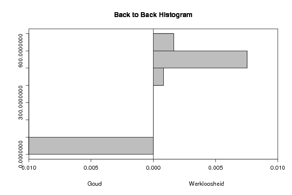
| Title produced by software | Back to Back Histogram | ||||||||||||||||||||
| Date of computation | Sun, 19 Oct 2008 11:48:30 -0600 | ||||||||||||||||||||
| Cite this page as follows | Statistical Computations at FreeStatistics.org, Office for Research Development and Education, URL https://freestatistics.org/blog/index.php?v=date/2008/Oct/19/t1224438542mzl3d7ixpi4xn6o.htm/, Retrieved Sun, 19 May 2024 15:26:34 +0000 | ||||||||||||||||||||
| Statistical Computations at FreeStatistics.org, Office for Research Development and Education, URL https://freestatistics.org/blog/index.php?pk=17008, Retrieved Sun, 19 May 2024 15:26:34 +0000 | |||||||||||||||||||||
| QR Codes: | |||||||||||||||||||||
|
| |||||||||||||||||||||
| Original text written by user: | |||||||||||||||||||||
| IsPrivate? | No (this computation is public) | ||||||||||||||||||||
| User-defined keywords | |||||||||||||||||||||
| Estimated Impact | 141 | ||||||||||||||||||||
Tree of Dependent Computations | |||||||||||||||||||||
| Family? (F = Feedback message, R = changed R code, M = changed R Module, P = changed Parameters, D = changed Data) | |||||||||||||||||||||
| F [Back to Back Histogram] [Goud-werkloosheid] [2008-10-19 17:48:30] [7f3f68cb5622d7511b280fd3e248ef1b] [Current] | |||||||||||||||||||||
| Feedback Forum | |||||||||||||||||||||
Post a new message | |||||||||||||||||||||
Dataset | |||||||||||||||||||||
| Dataseries X: | |||||||||||||||||||||
10.846 10.413 10.709 10.662 10.570 10.297 10.635 10.872 10.296 10.383 10.431 10.574 10.653 10.805 10.872 10.625 10.407 10.463 10.556 10.646 10.702 11.353 11.346 11.451 11.964 12.574 13.031 13.812 14.544 14.931 14.886 16.005 17.064 15.168 16.050 15.839 15.137 14.954 15.648 15.305 15.579 16.348 15.928 16.171 15.937 15.713 15.594 15.683 16.438 17.032 17.696 17.745 19.394 20.148 20.108 18.584 18.441 18.391 19.178 18.079 18.483 | |||||||||||||||||||||
| Dataseries Y: | |||||||||||||||||||||
578 565 547 555 562 561 555 544 537 543 594 611 613 611 594 595 591 589 584 573 567 569 621 629 628 612 595 597 593 590 580 574 573 573 620 626 620 588 566 557 561 549 532 526 511 499 555 565 542 527 510 514 517 508 493 490 469 478 528 534 518 | |||||||||||||||||||||
Tables (Output of Computation) | |||||||||||||||||||||
| |||||||||||||||||||||
Figures (Output of Computation) | |||||||||||||||||||||
Input Parameters & R Code | |||||||||||||||||||||
| Parameters (Session): | |||||||||||||||||||||
| par1 = grey ; par2 = grey ; par3 = TRUE ; par4 = Goud ; par5 = Werkloosheid ; | |||||||||||||||||||||
| Parameters (R input): | |||||||||||||||||||||
| par1 = grey ; par2 = grey ; par3 = TRUE ; par4 = Goud ; par5 = Werkloosheid ; | |||||||||||||||||||||
| R code (references can be found in the software module): | |||||||||||||||||||||
if (par3 == 'TRUE') par3 <- TRUE | |||||||||||||||||||||