Free Statistics
of Irreproducible Research!
Description of Statistical Computation | |||||||||||||||||||||||||||||||||||||||||||||||||||||||||||||||||||||||||||||||||||||||||||||||||||
|---|---|---|---|---|---|---|---|---|---|---|---|---|---|---|---|---|---|---|---|---|---|---|---|---|---|---|---|---|---|---|---|---|---|---|---|---|---|---|---|---|---|---|---|---|---|---|---|---|---|---|---|---|---|---|---|---|---|---|---|---|---|---|---|---|---|---|---|---|---|---|---|---|---|---|---|---|---|---|---|---|---|---|---|---|---|---|---|---|---|---|---|---|---|---|---|---|---|---|---|
| Author's title | |||||||||||||||||||||||||||||||||||||||||||||||||||||||||||||||||||||||||||||||||||||||||||||||||||
| Author | *The author of this computation has been verified* | ||||||||||||||||||||||||||||||||||||||||||||||||||||||||||||||||||||||||||||||||||||||||||||||||||
| R Software Module | rwasp_correlation.wasp | ||||||||||||||||||||||||||||||||||||||||||||||||||||||||||||||||||||||||||||||||||||||||||||||||||
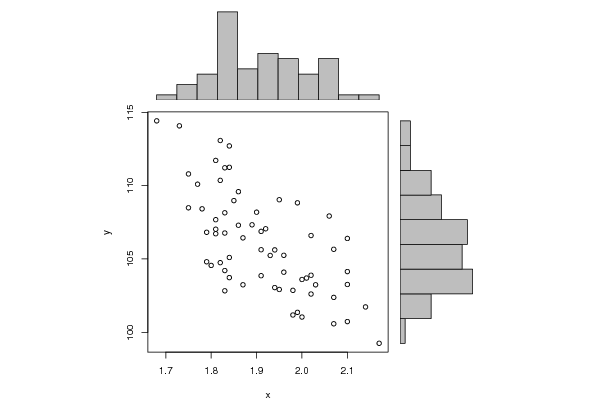
| Title produced by software | Pearson Correlation | ||||||||||||||||||||||||||||||||||||||||||||||||||||||||||||||||||||||||||||||||||||||||||||||||||
| Date of computation | Sat, 18 Oct 2008 07:27:30 -0600 | ||||||||||||||||||||||||||||||||||||||||||||||||||||||||||||||||||||||||||||||||||||||||||||||||||
| Cite this page as follows | Statistical Computations at FreeStatistics.org, Office for Research Development and Education, URL https://freestatistics.org/blog/index.php?v=date/2008/Oct/18/t122433661019jhyh2dqdnmfw6.htm/, Retrieved Sun, 19 May 2024 15:37:36 +0000 | ||||||||||||||||||||||||||||||||||||||||||||||||||||||||||||||||||||||||||||||||||||||||||||||||||
| Statistical Computations at FreeStatistics.org, Office for Research Development and Education, URL https://freestatistics.org/blog/index.php?pk=16617, Retrieved Sun, 19 May 2024 15:37:36 +0000 | |||||||||||||||||||||||||||||||||||||||||||||||||||||||||||||||||||||||||||||||||||||||||||||||||||
| QR Codes: | |||||||||||||||||||||||||||||||||||||||||||||||||||||||||||||||||||||||||||||||||||||||||||||||||||
|
| |||||||||||||||||||||||||||||||||||||||||||||||||||||||||||||||||||||||||||||||||||||||||||||||||||
| Original text written by user: | |||||||||||||||||||||||||||||||||||||||||||||||||||||||||||||||||||||||||||||||||||||||||||||||||||
| IsPrivate? | No (this computation is public) | ||||||||||||||||||||||||||||||||||||||||||||||||||||||||||||||||||||||||||||||||||||||||||||||||||
| User-defined keywords | |||||||||||||||||||||||||||||||||||||||||||||||||||||||||||||||||||||||||||||||||||||||||||||||||||
| Estimated Impact | 131 | ||||||||||||||||||||||||||||||||||||||||||||||||||||||||||||||||||||||||||||||||||||||||||||||||||
Tree of Dependent Computations | |||||||||||||||||||||||||||||||||||||||||||||||||||||||||||||||||||||||||||||||||||||||||||||||||||
| Family? (F = Feedback message, R = changed R code, M = changed R Module, P = changed Parameters, D = changed Data) | |||||||||||||||||||||||||||||||||||||||||||||||||||||||||||||||||||||||||||||||||||||||||||||||||||
| F [Univariate Data Series] [Eerste tijdreeks] [2008-10-11 15:49:53] [c45c87b96bbf32ffc2144fc37d767b2e] - PD [Univariate Data Series] [aantal begonnen w...] [2008-10-18 13:04:32] [c45c87b96bbf32ffc2144fc37d767b2e] F RMPD [Pearson Correlation] [relatie tijdreeks...] [2008-10-18 13:27:30] [3dc594a6c62226e1e98766c4d385bfaa] [Current] F D [Pearson Correlation] [relatie tijdreeks...] [2008-10-18 13:31:33] [c45c87b96bbf32ffc2144fc37d767b2e] F D [Pearson Correlation] [relatie tijdreeks...] [2008-10-18 13:35:31] [c45c87b96bbf32ffc2144fc37d767b2e] F D [Pearson Correlation] [relatie tijdreeks...] [2008-10-18 13:37:37] [c45c87b96bbf32ffc2144fc37d767b2e] F D [Pearson Correlation] [relatie tijdreeks...] [2008-10-18 13:39:20] [c45c87b96bbf32ffc2144fc37d767b2e] F D [Pearson Correlation] [relatie tijdreeks...] [2008-10-18 13:41:34] [c45c87b96bbf32ffc2144fc37d767b2e] | |||||||||||||||||||||||||||||||||||||||||||||||||||||||||||||||||||||||||||||||||||||||||||||||||||
| Feedback Forum | |||||||||||||||||||||||||||||||||||||||||||||||||||||||||||||||||||||||||||||||||||||||||||||||||||
Post a new message | |||||||||||||||||||||||||||||||||||||||||||||||||||||||||||||||||||||||||||||||||||||||||||||||||||
Dataset | |||||||||||||||||||||||||||||||||||||||||||||||||||||||||||||||||||||||||||||||||||||||||||||||||||
| Dataseries X: | |||||||||||||||||||||||||||||||||||||||||||||||||||||||||||||||||||||||||||||||||||||||||||||||||||
1.83 1.91 1.68 1.82 1.75 1.83 1.73 1.81 2.10 1.90 1.91 2.02 1.99 1.96 1.81 1.75 1.82 2.00 1.91 1.84 1.83 1.94 1.83 1.79 1.98 1.95 1.81 1.79 1.84 1.89 1.78 1.84 2.00 1.87 1.98 2.02 2.10 1.99 1.77 1.83 1.94 1.80 1.92 1.85 2.10 2.03 2.07 2.10 2.14 2.17 1.93 1.87 2.07 1.86 1.82 1.95 2.02 2.01 2.06 2.07 1.86 1.96 1.81 1.84 | |||||||||||||||||||||||||||||||||||||||||||||||||||||||||||||||||||||||||||||||||||||||||||||||||||
| Dataseries Y: | |||||||||||||||||||||||||||||||||||||||||||||||||||||||||||||||||||||||||||||||||||||||||||||||||||
104.21 103.86 114.42 113.08 110.80 111.22 114.08 111.72 106.40 108.19 106.88 106.60 108.83 104.10 107.03 108.49 104.75 101.04 105.63 105.10 108.15 105.62 102.83 104.81 102.86 102.92 107.68 106.82 103.73 107.33 108.42 111.25 103.60 103.24 101.18 102.61 104.14 101.36 110.10 106.77 103.05 104.56 107.06 108.98 103.26 103.24 100.58 100.73 101.73 99.25 105.24 106.44 105.66 109.59 110.36 109.04 103.89 103.70 107.93 102.38 107.30 105,25 106.72 112.71 | |||||||||||||||||||||||||||||||||||||||||||||||||||||||||||||||||||||||||||||||||||||||||||||||||||
Tables (Output of Computation) | |||||||||||||||||||||||||||||||||||||||||||||||||||||||||||||||||||||||||||||||||||||||||||||||||||
| |||||||||||||||||||||||||||||||||||||||||||||||||||||||||||||||||||||||||||||||||||||||||||||||||||
Figures (Output of Computation) | |||||||||||||||||||||||||||||||||||||||||||||||||||||||||||||||||||||||||||||||||||||||||||||||||||
Input Parameters & R Code | |||||||||||||||||||||||||||||||||||||||||||||||||||||||||||||||||||||||||||||||||||||||||||||||||||
| Parameters (Session): | |||||||||||||||||||||||||||||||||||||||||||||||||||||||||||||||||||||||||||||||||||||||||||||||||||
| Parameters (R input): | |||||||||||||||||||||||||||||||||||||||||||||||||||||||||||||||||||||||||||||||||||||||||||||||||||
| R code (references can be found in the software module): | |||||||||||||||||||||||||||||||||||||||||||||||||||||||||||||||||||||||||||||||||||||||||||||||||||
bitmap(file='test1.png') | |||||||||||||||||||||||||||||||||||||||||||||||||||||||||||||||||||||||||||||||||||||||||||||||||||