Free Statistics
of Irreproducible Research!
Description of Statistical Computation | |||||||||||||||||||||||||||||||||||||||||
|---|---|---|---|---|---|---|---|---|---|---|---|---|---|---|---|---|---|---|---|---|---|---|---|---|---|---|---|---|---|---|---|---|---|---|---|---|---|---|---|---|---|
| Author's title | |||||||||||||||||||||||||||||||||||||||||
| Author | *The author of this computation has been verified* | ||||||||||||||||||||||||||||||||||||||||
| R Software Module | rwasp_univariatedataseries.wasp | ||||||||||||||||||||||||||||||||||||||||
| Title produced by software | Univariate Data Series | ||||||||||||||||||||||||||||||||||||||||
| Date of computation | Mon, 13 Oct 2008 09:28:04 -0600 | ||||||||||||||||||||||||||||||||||||||||
| Cite this page as follows | Statistical Computations at FreeStatistics.org, Office for Research Development and Education, URL https://freestatistics.org/blog/index.php?v=date/2008/Oct/13/t1223911734q8frqxhfy5feh9k.htm/, Retrieved Sun, 19 May 2024 13:34:14 +0000 | ||||||||||||||||||||||||||||||||||||||||
| Statistical Computations at FreeStatistics.org, Office for Research Development and Education, URL https://freestatistics.org/blog/index.php?pk=15659, Retrieved Sun, 19 May 2024 13:34:14 +0000 | |||||||||||||||||||||||||||||||||||||||||
| QR Codes: | |||||||||||||||||||||||||||||||||||||||||
|
| |||||||||||||||||||||||||||||||||||||||||
| Original text written by user: | |||||||||||||||||||||||||||||||||||||||||
| IsPrivate? | No (this computation is public) | ||||||||||||||||||||||||||||||||||||||||
| User-defined keywords | |||||||||||||||||||||||||||||||||||||||||
| Estimated Impact | 269 | ||||||||||||||||||||||||||||||||||||||||
Tree of Dependent Computations | |||||||||||||||||||||||||||||||||||||||||
| Family? (F = Feedback message, R = changed R code, M = changed R Module, P = changed Parameters, D = changed Data) | |||||||||||||||||||||||||||||||||||||||||
| F [Univariate Data Series] [Werkloosheid mannen] [2008-10-13 15:28:04] [35348cd8592af0baf5f138bd59921307] [Current] - RMPD [Central Tendency] [Central tendency ...] [2008-10-20 13:22:34] [7d3039e6253bb5fb3b26df1537d500b4] - RMPD [Percentiles] [Percentiles reeks 1] [2008-10-20 13:29:02] [7d3039e6253bb5fb3b26df1537d500b4] - RMPD [Stem-and-leaf Plot] [Stem and leaf ree...] [2008-10-20 13:31:06] [7d3039e6253bb5fb3b26df1537d500b4] - RMPD [Histogram] [Histogram reeks 1] [2008-10-20 13:34:27] [7d3039e6253bb5fb3b26df1537d500b4] - RMPD [Harrell-Davis Quantiles] [Harell-davis reeks 1] [2008-10-20 13:36:57] [7d3039e6253bb5fb3b26df1537d500b4] F RMPD [Back to Back Histogram] [Back to back reeks 1] [2008-10-20 13:39:56] [7d3039e6253bb5fb3b26df1537d500b4] - PD [Back to Back Histogram] [Q8 Back to back m...] [2008-10-27 19:38:08] [7d3039e6253bb5fb3b26df1537d500b4] - PD [Back to Back Histogram] [Q8 back to back m...] [2008-10-27 19:50:07] [7d3039e6253bb5fb3b26df1537d500b4] - PD [Back to Back Histogram] [Q8 back to back m...] [2008-10-27 19:52:12] [7d3039e6253bb5fb3b26df1537d500b4] - PD [Back to Back Histogram] [Q8 back to back v...] [2008-10-27 19:54:13] [7d3039e6253bb5fb3b26df1537d500b4] - PD [Back to Back Histogram] [Q8 back to back v...] [2008-10-27 19:55:33] [7d3039e6253bb5fb3b26df1537d500b4] - PD [Back to Back Histogram] [Q8 back to back j...] [2008-10-27 19:56:53] [7d3039e6253bb5fb3b26df1537d500b4] - RMPD [Pearson Correlation] [Pearson correlati...] [2008-10-20 13:44:24] [7d3039e6253bb5fb3b26df1537d500b4] - PD [Univariate Data Series] [] [2008-10-20 14:53:04] [af90f76a5211a482a7c35f2c76d2fd61] - RMPD [Central Tendency] [] [2008-10-26 15:32:39] [af90f76a5211a482a7c35f2c76d2fd61] - RMP [Stem-and-leaf Plot] [] [2008-10-26 15:35:41] [af90f76a5211a482a7c35f2c76d2fd61] - RMPD [Percentiles] [] [2008-10-26 15:38:00] [af90f76a5211a482a7c35f2c76d2fd61] - RMP [Harrell-Davis Quantiles] [] [2008-10-26 15:40:03] [af90f76a5211a482a7c35f2c76d2fd61] - RMPD [Central Tendency] [] [2008-10-26 15:42:50] [af90f76a5211a482a7c35f2c76d2fd61] - RM D [Stem-and-leaf Plot] [] [2008-10-26 15:44:02] [af90f76a5211a482a7c35f2c76d2fd61] - RM [Percentiles] [] [2008-10-26 15:45:16] [af90f76a5211a482a7c35f2c76d2fd61] - RM [Harrell-Davis Quantiles] [] [2008-10-26 15:46:52] [af90f76a5211a482a7c35f2c76d2fd61] - RM D [Central Tendency] [] [2008-10-26 15:49:47] [af90f76a5211a482a7c35f2c76d2fd61] - RM D [Stem-and-leaf Plot] [] [2008-10-26 15:51:02] [af90f76a5211a482a7c35f2c76d2fd61] - RM [Percentiles] [] [2008-10-26 15:52:22] [af90f76a5211a482a7c35f2c76d2fd61] - RM [Harrell-Davis Quantiles] [] [2008-10-26 15:53:29] [af90f76a5211a482a7c35f2c76d2fd61] - RM D [Central Tendency] [] [2008-10-26 15:55:24] [af90f76a5211a482a7c35f2c76d2fd61] - RM D [Stem-and-leaf Plot] [] [2008-10-26 15:56:53] [af90f76a5211a482a7c35f2c76d2fd61] - RM [Percentiles] [] [2008-10-26 15:58:01] [af90f76a5211a482a7c35f2c76d2fd61] - RM [Harrell-Davis Quantiles] [] [2008-10-26 15:59:16] [af90f76a5211a482a7c35f2c76d2fd61] - PD [Univariate Data Series] [] [2008-10-20 14:56:29] [af90f76a5211a482a7c35f2c76d2fd61] - PD [Univariate Data Series] [] [2008-10-20 14:58:15] [af90f76a5211a482a7c35f2c76d2fd61] - PD [Univariate Data Series] [] [2008-10-20 14:59:51] [af90f76a5211a482a7c35f2c76d2fd61] - PD [Univariate Data Series] [Aantal bouwvergun...] [2008-10-21 04:36:06] [645b47e0eb1e1e0301fa1dba1a86991a] - PD [Univariate Data Series] [Productie woningen] [2008-10-21 04:38:40] [645b47e0eb1e1e0301fa1dba1a86991a] | |||||||||||||||||||||||||||||||||||||||||
| Feedback Forum | |||||||||||||||||||||||||||||||||||||||||
Post a new message | |||||||||||||||||||||||||||||||||||||||||
Dataset | |||||||||||||||||||||||||||||||||||||||||
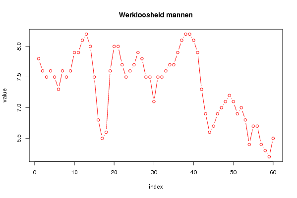
| Dataseries X: | |||||||||||||||||||||||||||||||||||||||||
7,8 7,6 7,5 7,6 7,5 7,3 7,6 7,5 7,6 7,9 7,9 8,1 8,2 8,0 7,5 6,8 6,5 6,6 7,6 8,0 8,0 7,7 7,5 7,6 7,7 7,9 7,8 7,5 7,5 7,1 7,5 7,5 7,6 7,7 7,7 7,9 8,1 8,2 8,2 8,1 7,9 7,3 6,9 6,6 6,7 6,9 7,0 7,1 7,2 7,1 6,9 7,0 6,8 6,4 6,7 6,7 6,4 6,3 6,2 6,5 | |||||||||||||||||||||||||||||||||||||||||
Tables (Output of Computation) | |||||||||||||||||||||||||||||||||||||||||
| |||||||||||||||||||||||||||||||||||||||||
Figures (Output of Computation) | |||||||||||||||||||||||||||||||||||||||||
Input Parameters & R Code | |||||||||||||||||||||||||||||||||||||||||
| Parameters (Session): | |||||||||||||||||||||||||||||||||||||||||
| par1 = Werkloosheid mannen ; | |||||||||||||||||||||||||||||||||||||||||
| Parameters (R input): | |||||||||||||||||||||||||||||||||||||||||
| par1 = Werkloosheid mannen ; par2 = ; par3 = ; | |||||||||||||||||||||||||||||||||||||||||
| R code (references can be found in the software module): | |||||||||||||||||||||||||||||||||||||||||
bitmap(file='test1.png') | |||||||||||||||||||||||||||||||||||||||||