Free Statistics
of Irreproducible Research!
Description of Statistical Computation | |||||||||||||||||||||||||||||||||
|---|---|---|---|---|---|---|---|---|---|---|---|---|---|---|---|---|---|---|---|---|---|---|---|---|---|---|---|---|---|---|---|---|---|
| Author's title | |||||||||||||||||||||||||||||||||
| Author | *The author of this computation has been verified* | ||||||||||||||||||||||||||||||||
| R Software Module | rwasp_density.wasp | ||||||||||||||||||||||||||||||||
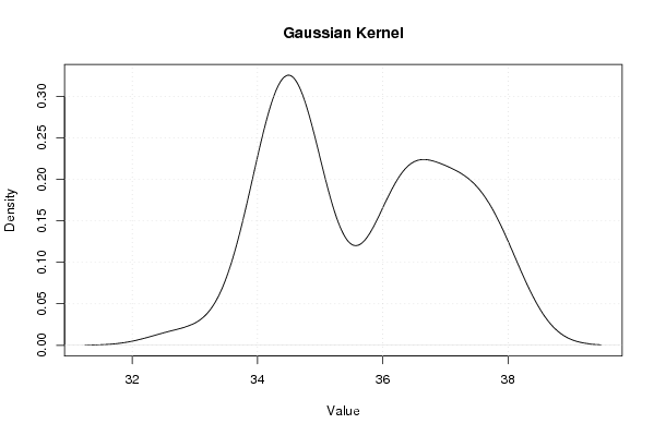
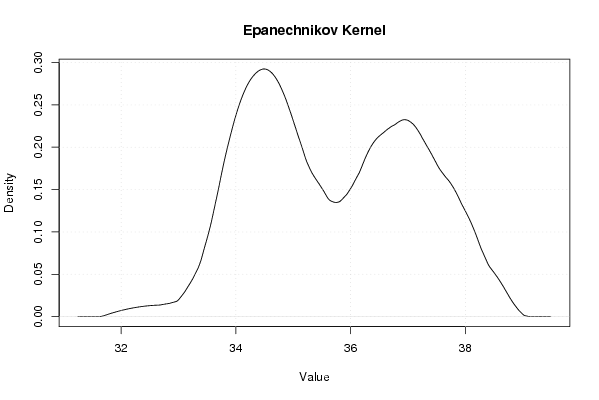
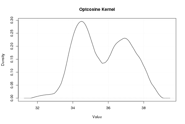
| Title produced by software | Kernel Density Estimation | ||||||||||||||||||||||||||||||||
| Date of computation | Sun, 12 Oct 2008 11:48:20 -0600 | ||||||||||||||||||||||||||||||||
| Cite this page as follows | Statistical Computations at FreeStatistics.org, Office for Research Development and Education, URL https://freestatistics.org/blog/index.php?v=date/2008/Oct/12/t1223833784ac5clq6c67mz8sg.htm/, Retrieved Sun, 19 May 2024 13:22:14 +0000 | ||||||||||||||||||||||||||||||||
| Statistical Computations at FreeStatistics.org, Office for Research Development and Education, URL https://freestatistics.org/blog/index.php?pk=15512, Retrieved Sun, 19 May 2024 13:22:14 +0000 | |||||||||||||||||||||||||||||||||
| QR Codes: | |||||||||||||||||||||||||||||||||
|
| |||||||||||||||||||||||||||||||||
| Original text written by user: | |||||||||||||||||||||||||||||||||
| IsPrivate? | No (this computation is public) | ||||||||||||||||||||||||||||||||
| User-defined keywords | |||||||||||||||||||||||||||||||||
| Estimated Impact | 169 | ||||||||||||||||||||||||||||||||
Tree of Dependent Computations | |||||||||||||||||||||||||||||||||
| Family? (F = Feedback message, R = changed R code, M = changed R Module, P = changed Parameters, D = changed Data) | |||||||||||||||||||||||||||||||||
| - [Univariate Data Series] [Prijsevolutie ver...] [2008-10-06 10:26:50] [a18c43c8b63fa6800a53bb187b9ddd45] - RMPD [Kernel Density Estimation] [Dichtheidsgrafiek...] [2008-10-12 17:48:20] [768ad88abce8b6ce0be22cfe8ac9beaf] [Current] - RM D [Quartiles] [kwartielen maximu...] [2008-10-12 18:15:14] [a18c43c8b63fa6800a53bb187b9ddd45] - RMPD [Notched Boxplots] [Boxplot maximumpr...] [2008-10-12 18:17:15] [a18c43c8b63fa6800a53bb187b9ddd45] | |||||||||||||||||||||||||||||||||
| Feedback Forum | |||||||||||||||||||||||||||||||||
Post a new message | |||||||||||||||||||||||||||||||||
Dataset | |||||||||||||||||||||||||||||||||
| Dataseries X: | |||||||||||||||||||||||||||||||||
34.1 34.11 34.11 34.11 34.11 34.23 34.23 34.19 34.38 34.69 34.69 34.69 34.69 34.69 34.69 34.63 34.63 34.63 34.63 33.8 32.75 34.08 34.36 34.36 34.48 34.48 34.52 34.52 34.52 34.52 34.52 33.98 32.8 34.3 34.43 34.48 34.48 34.48 34.48 34.74 34.82 34.82 34.82 34.82 34.75 35.93 36.2 36.2 36.21 36.31 36.34 36.36 36.42 36.45 36.45 35.46 34.81 36.05 36.12 36.13 36.15 36.51 36.52 36.54 36.39 36.43 36.42 36.26 36.8 36.85 37.15 37.15 37.15 37.19 37.28 37.28 37.28 37.27 37.28 37.33 36.82 37.3 37.62 37.67 37.74 37.81 37.9 37.89 37.7 37.89 37.9 37.14 36.82 37.8 37.94 37.99 | |||||||||||||||||||||||||||||||||
Tables (Output of Computation) | |||||||||||||||||||||||||||||||||
| |||||||||||||||||||||||||||||||||
Figures (Output of Computation) | |||||||||||||||||||||||||||||||||
Input Parameters & R Code | |||||||||||||||||||||||||||||||||
| Parameters (Session): | |||||||||||||||||||||||||||||||||
| Parameters (R input): | |||||||||||||||||||||||||||||||||
| R code (references can be found in the software module): | |||||||||||||||||||||||||||||||||
bitmap(file='density1.png') | |||||||||||||||||||||||||||||||||