Free Statistics

of Irreproducible Research!

Author's title

Author*Unverified author*
R Software Modulerwasp_babies.wasp
Title produced by softwareExercise 1.13
Date of computationFri, 10 Oct 2008 08:20:35 -0600
Cite this page as followsStatistical Computations at FreeStatistics.org, Office for Research Development and Education, URL https://freestatistics.org/blog/index.php?v=date/2008/Oct/10/t1223648475mwof604kcbepncq.htm/, Retrieved Sun, 19 May 2024 19:49:21 +0000
Statistical Computations at FreeStatistics.org, Office for Research Development and Education, URL https://freestatistics.org/blog/index.php?pk=15235, Retrieved Sun, 19 May 2024 19:49:21 +0000
QR Codes:

Original text written by user:
IsPrivate?No (this computation is public)
User-defined keywordsBabies exercise 1.13 timeshift
Estimated Impact186
Family? (F = Feedback message, R = changed R code, M = changed R Module, P = changed Parameters, D = changed Data)
F     [Exercise 1.13] [Exercise 1.13 (Wo...] [2008-10-01 13:28:34] [b98453cac15ba1066b407e146608df68]
F   P     [Exercise 1.13] [Babies2] [2008-10-10 14:20:35] [d41d8cd98f00b204e9800998ecf8427e] [Current]
Feedback Forum
2008-10-18 10:54:58 [e117fb22a86bc68899e345062e1db29a] [reply
De oplossing die werd gegeven is volledig correct. De student heeft als eerste link de grafieken toegevoegd waarbij er slechts gedurende 365 dagen werd geobserveerd, in deze grafieken is te zien dat de curve niet stabiel is en de waarschijnlijkheid relatief hoog.
In de tweede link: http://www.freestatistics.org/blog/index.php?v=date/2008/Oct/10/t1223648475mwof604kcbepncq.htm werd bewezen dat naarmate men de tijdspanne van de steekproef verhoogt, zoals in dit voorbeeld 2920 dagen, de curve stabiliseert en de waarschijnlijkheid verkleint. Door de tijdspanne te verhogen zal de nauwkeurigheid van de metingen verbeteren en de schommelingen verkleinen, waardoor uiteindelijk het resultaat slechts 0.139% bedraagt.
2008-10-19 16:36:06 [Yara Van Overstraeten] [reply
In een vorige link (http://www.freestatistics.org/blog/index.php?v=date/2008/Oct/10/t1223648131bu39ufcgaovja8l.htm) was de student tot het besluit gekomen dat de resultaten te hard schommelden om accuraat te zijn. Hij/zij is dan tot het besluit gekomen dat men de tijdspanne waarin de resulaten worden berekend dient te verlengen om een stabieler cijfer te verkrijgen. Hij heeft het aantal dagen verhoogt van 365 naar 2920 dagen en bekomt hier een resultaat van 13,97%. De student heeft dus een correcte oplossing gegeven op deze vraag.
2008-10-19 20:40:36 [Stéphanie Thijs] [reply
Het resultaat kan nog nauwkeuriger door de parameter van het aantal gesimuleerde dagen naar 3650 te verhogen.
2008-10-20 17:16:36 [Jeroen Aerts] [reply
De grafiek toont meteen aan wat de oplossing betekent en is ook volledig correct. De student begrijpt de vraag en geeft een duidelijke gestructureerde oplossing.

Post a new message


Summary of computational transaction
Raw Inputview raw input (R code)
Raw Outputview raw output of R engine
Computing time3 seconds
R Server'George Udny Yule' @ 72.249.76.132

\begin{tabular}{lllllllll}
\hline
Summary of computational transaction \tabularnewline
Raw Input & view raw input (R code)  \tabularnewline
Raw Output & view raw output of R engine  \tabularnewline
Computing time & 3 seconds \tabularnewline
R Server & 'George Udny Yule' @ 72.249.76.132 \tabularnewline
\hline
\end{tabular}
%Source: https://freestatistics.org/blog/index.php?pk=15235&T=0

[TABLE]
[ROW][C]Summary of computational transaction[/C][/ROW]
[ROW][C]Raw Input[/C][C]view raw input (R code) [/C][/ROW]
[ROW][C]Raw Output[/C][C]view raw output of R engine [/C][/ROW]
[ROW][C]Computing time[/C][C]3 seconds[/C][/ROW]
[ROW][C]R Server[/C][C]'George Udny Yule' @ 72.249.76.132[/C][/ROW]
[/TABLE]
Source: https://freestatistics.org/blog/index.php?pk=15235&T=0

Globally Unique Identifier (entire table): ba.freestatistics.org/blog/index.php?pk=15235&T=0

As an alternative you can also use a QR Code:  

The GUIDs for individual cells are displayed in the table below:

Summary of computational transaction
Raw Inputview raw input (R code)
Raw Outputview raw output of R engine
Computing time3 seconds
R Server'George Udny Yule' @ 72.249.76.132


Exercise 1.13 p. 14 (Introduction to Probability, 2nd ed.)
Number of simulated days2920
Expected number of births in Large Hospital45
Expected number of births in Small Hospital15
Percentage of Male births per day(for which the probability is computed)0.6
#Females births in Large Hospital65717
#Males births in Large Hospital65683
#Female births in Small Hospital21989
#Male births in Small Hospital21811
Probability of more than 60 % of male births in Large Hospital0.0657534246575342
Probability of more than 60 % of male births in Small Hospital0.139726027397260
#Days per Year when more than 60 % of male births occur in Large Hospital24
#Days per Year when more than 60 % of male births occur in Small Hospital51

\begin{tabular}{lllllllll}
\hline
Exercise 1.13 p. 14 (Introduction to Probability, 2nd ed.) \tabularnewline
Number of simulated days & 2920 \tabularnewline
Expected number of births in Large Hospital & 45 \tabularnewline
Expected number of births in Small Hospital & 15 \tabularnewline
Percentage of Male births per day(for which the probability is computed) & 0.6 \tabularnewline
#Females births in Large Hospital & 65717 \tabularnewline
#Males births in Large Hospital & 65683 \tabularnewline
#Female births in Small Hospital & 21989 \tabularnewline
#Male births in Small Hospital & 21811 \tabularnewline
Probability of more than 60 % of male births in Large Hospital & 0.0657534246575342 \tabularnewline
Probability of more than 60 % of male births in Small Hospital & 0.139726027397260 \tabularnewline
#Days per Year when more than 60 % of male births occur in Large Hospital & 24 \tabularnewline
#Days per Year when more than 60 % of male births occur in Small Hospital & 51 \tabularnewline
\hline
\end{tabular}
%Source: https://freestatistics.org/blog/index.php?pk=15235&T=1

[TABLE]
[ROW][C]Exercise 1.13 p. 14 (Introduction to Probability, 2nd ed.)[/C][/ROW]
[ROW][C]Number of simulated days[/C][C]2920[/C][/ROW]
[ROW][C]Expected number of births in Large Hospital[/C][C]45[/C][/ROW]
[ROW][C]Expected number of births in Small Hospital[/C][C]15[/C][/ROW]
[ROW][C]Percentage of Male births per day(for which the probability is computed)[/C][C]0.6[/C][/ROW]
[ROW][C]#Females births in Large Hospital[/C][C]65717[/C][/ROW]
[ROW][C]#Males births in Large Hospital[/C][C]65683[/C][/ROW]
[ROW][C]#Female births in Small Hospital[/C][C]21989[/C][/ROW]
[ROW][C]#Male births in Small Hospital[/C][C]21811[/C][/ROW]
[ROW][C]Probability of more than 60 % of male births in Large Hospital[/C][C]0.0657534246575342[/C][/ROW]
[C]Probability of more than 60 % of male births in Small Hospital[/C][C]0.139726027397260[/C][/ROW]
[ROW][C]#Days per Year when more than 60 % of male births occur in Large Hospital[/C][C]24[/C][/ROW]
[C]#Days per Year when more than 60 % of male births occur in Small Hospital[/C][C]51[/C][/ROW]
[/TABLE]
Source: https://freestatistics.org/blog/index.php?pk=15235&T=1

Globally Unique Identifier (entire table): ba.freestatistics.org/blog/index.php?pk=15235&T=1

As an alternative you can also use a QR Code:  

The GUIDs for individual cells are displayed in the table below:

Exercise 1.13 p. 14 (Introduction to Probability, 2nd ed.)
Number of simulated days2920
Expected number of births in Large Hospital45
Expected number of births in Small Hospital15
Percentage of Male births per day(for which the probability is computed)0.6
#Females births in Large Hospital65717
#Males births in Large Hospital65683
#Female births in Small Hospital21989
#Male births in Small Hospital21811
Probability of more than 60 % of male births in Large Hospital0.0657534246575342
Probability of more than 60 % of male births in Small Hospital0.139726027397260
#Days per Year when more than 60 % of male births occur in Large Hospital24
#Days per Year when more than 60 % of male births occur in Small Hospital51


Parameters (Session):
par1 = 730 ; par2 = 45 ; par3 = 15 ; par4 = 0.6 ;
Parameters (R input):
par1 = 2920 ; par2 = 45 ; par3 = 15 ; par4 = 0.6 ;
R code (references can be found in the software module):
par1 <- as.numeric(par1)
par2 <- as.numeric(par2)
par3 <- as.numeric(par3)
par4 <- as.numeric(par4)
numsuccessbig <- 0
numsuccesssmall <- 0
bighospital <- array(NA,dim=c(par1,par2))
smallhospital <- array(NA,dim=c(par1,par3))
bigprob <- array(NA,dim=par1)
smallprob <- array(NA,dim=par1)
for (i in 1:par1) {
bighospital[i,] <- sample(c('F','M'),par2,replace=TRUE)
if (as.matrix(table(bighospital[i,]))[2] > par4*par2) numsuccessbig = numsuccessbig + 1
bigprob[i] <- numsuccessbig/i
smallhospital[i,] <- sample(c('F','M'),par3,replace=TRUE)
if (as.matrix(table(smallhospital[i,]))[2] > par4*par3) numsuccesssmall = numsuccesssmall + 1
smallprob[i] <- numsuccesssmall/i
}
tbig <- as.matrix(table(bighospital))
tsmall <- as.matrix(table(smallhospital))
tbig
tsmall
numsuccessbig/par1
bigprob[par1]
numsuccesssmall/par1
smallprob[par1]
numsuccessbig/par1*365
bigprob[par1]*365
numsuccesssmall/par1*365
smallprob[par1]*365
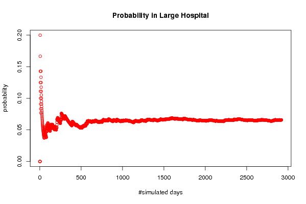
bitmap(file='test1.png')
plot(bigprob,col=2,main='Probability in Large Hospital',xlab='#simulated days',ylab='probability')
dev.off()
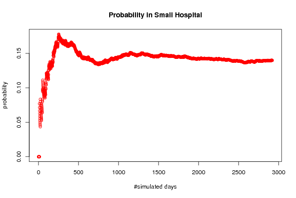
bitmap(file='test2.png')
plot(smallprob,col=2,main='Probability in Small Hospital',xlab='#simulated days',ylab='probability')
dev.off()
load(file='createtable')
a<-table.start()
a<-table.row.start(a)
a<-table.element(a,'Exercise 1.13 p. 14 (Introduction to Probability, 2nd ed.)',2,TRUE)
a<-table.row.end(a)
a<-table.row.start(a)
a<-table.element(a,'Number of simulated days',header=TRUE)
a<-table.element(a,par1)
a<-table.row.end(a)
a<-table.row.start(a)
a<-table.element(a,'Expected number of births in Large Hospital',header=TRUE)
a<-table.element(a,par2)
a<-table.row.end(a)
a<-table.row.start(a)
a<-table.element(a,'Expected number of births in Small Hospital',header=TRUE)
a<-table.element(a,par3)
a<-table.row.end(a)
a<-table.row.start(a)
a<-table.element(a,'Percentage of Male births per day
(for which the probability is computed)',header=TRUE)
a<-table.element(a,par4)
a<-table.row.end(a)
a<-table.row.start(a)
a<-table.element(a,'#Females births in Large Hospital',header=TRUE)
a<-table.element(a,tbig[1])
a<-table.row.end(a)
a<-table.row.start(a)
a<-table.element(a,'#Males births in Large Hospital',header=TRUE)
a<-table.element(a,tbig[2])
a<-table.row.end(a)
a<-table.row.start(a)
a<-table.element(a,'#Female births in Small Hospital',header=TRUE)
a<-table.element(a,tsmall[1])
a<-table.row.end(a)
a<-table.row.start(a)
a<-table.element(a,'#Male births in Small Hospital',header=TRUE)
a<-table.element(a,tsmall[2])
a<-table.row.end(a)
a<-table.row.start(a)
dum1 <- paste('Probability of more than', par4*100, sep=' ')
dum <- paste(dum1, '% of male births in Large Hospital', sep=' ')
a<-table.element(a, dum, header=TRUE)
a<-table.element(a, bigprob[par1])
a<-table.row.end(a)
dum <- paste(dum1, '% of male births in Small Hospital', sep=' ')
a<-table.element(a, dum, header=TRUE)
a<-table.element(a, smallprob[par1])
a<-table.row.end(a)
a<-table.row.start(a)
dum1 <- paste('#Days per Year when more than', par4*100, sep=' ')
dum <- paste(dum1, '% of male births occur in Large Hospital', sep=' ')
a<-table.element(a, dum, header=TRUE)
a<-table.element(a, bigprob[par1]*365)
a<-table.row.end(a)
dum <- paste(dum1, '% of male births occur in Small Hospital', sep=' ')
a<-table.element(a, dum, header=TRUE)
a<-table.element(a, smallprob[par1]*365)
a<-table.row.end(a)
a<-table.end(a)
table.save(a,file='mytable.tab')