\begin{tabular}{lllllllll}
\hline
Summary of computational transaction \tabularnewline
Raw Input & view raw input (R code)  \tabularnewline
Raw Output & view raw output of R engine  \tabularnewline
Computing time & 1 seconds \tabularnewline
R Server & 'Gwilym Jenkins' @ 72.249.127.135 \tabularnewline
\hline
\end{tabular}
%Source: https://freestatistics.org/blog/index.php?pk=14933&T=0
[TABLE]
[ROW][C]Summary of computational transaction[/C][/ROW]
[ROW][C]Raw Input[/C][C]view raw input (R code) [/C][/ROW]
[ROW][C]Raw Output[/C][C]view raw output of R engine [/C][/ROW]
[ROW][C]Computing time[/C][C]1 seconds[/C][/ROW]
[ROW][C]R Server[/C][C]'Gwilym Jenkins' @ 72.249.127.135[/C][/ROW]
[/TABLE]
Source: https://freestatistics.org/blog/index.php?pk=14933&T=0
If you paste this QR Code into your document, anyone with a smartphone or tablet will be able to scan it and view this table in a browser.
If you paste this QR Code into your document, anyone with a smartphone or tablet will be able to scan it and view this table in a browser.
If you paste this QR Code into your document, anyone with a smartphone or tablet will be able to scan it and view this table in a browser.
If you paste this QR Code into your document, anyone with a smartphone or tablet will be able to scan it and view this table in a browser.
If you paste this QR Code into your document, anyone with a smartphone or tablet will be able to scan it and view this table in a browser.
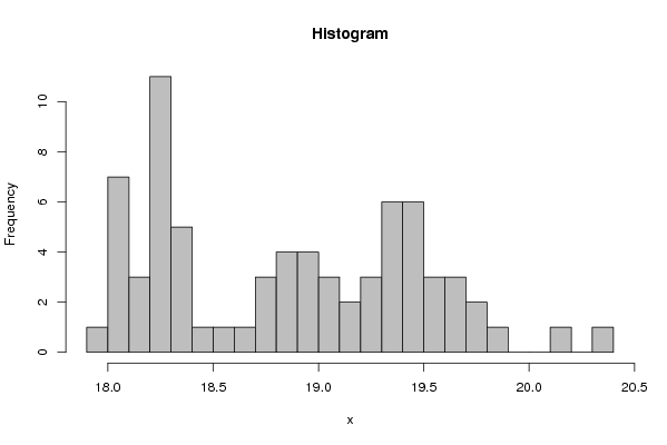
| Frequency Table (Histogram) | | Bins | Midpoint | Abs. Frequency | Rel. Frequency | Cumul. Rel. Freq. | Density | | [17.9,18[ | 17.95 | 1 | 0.013889 | 0.013889 | 0.138889 | | [18,18.1[ | 18.05 | 7 | 0.097222 | 0.111111 | 0.972222 | | [18.1,18.2[ | 18.15 | 3 | 0.041667 | 0.152778 | 0.416667 | | [18.2,18.3[ | 18.25 | 11 | 0.152778 | 0.305556 | 1.527778 | | [18.3,18.4[ | 18.35 | 5 | 0.069444 | 0.375 | 0.694444 | | [18.4,18.5[ | 18.45 | 1 | 0.013889 | 0.388889 | 0.138889 | | [18.5,18.6[ | 18.55 | 1 | 0.013889 | 0.402778 | 0.138889 | | [18.6,18.7[ | 18.65 | 1 | 0.013889 | 0.416667 | 0.138889 | | [18.7,18.8[ | 18.75 | 3 | 0.041667 | 0.458333 | 0.416667 | | [18.8,18.9[ | 18.85 | 4 | 0.055556 | 0.513889 | 0.555556 | | [18.9,19[ | 18.95 | 4 | 0.055556 | 0.569444 | 0.555556 | | [19,19.1[ | 19.05 | 3 | 0.041667 | 0.611111 | 0.416667 | | [19.1,19.2[ | 19.15 | 2 | 0.027778 | 0.638889 | 0.277778 | | [19.2,19.3[ | 19.25 | 3 | 0.041667 | 0.680556 | 0.416667 | | [19.3,19.4[ | 19.35 | 6 | 0.083333 | 0.763889 | 0.833333 | | [19.4,19.5[ | 19.45 | 6 | 0.083333 | 0.847222 | 0.833333 | | [19.5,19.6[ | 19.55 | 3 | 0.041667 | 0.888889 | 0.416667 | | [19.6,19.7[ | 19.65 | 3 | 0.041667 | 0.930556 | 0.416667 | | [19.7,19.8[ | 19.75 | 2 | 0.027778 | 0.958333 | 0.277778 | | [19.8,19.9[ | 19.85 | 1 | 0.013889 | 0.972222 | 0.138889 | | [19.9,20[ | 19.95 | 0 | 0 | 0.972222 | 0 | | [20,20.1[ | 20.05 | 0 | 0 | 0.972222 | 0 | | [20.1,20.2[ | 20.15 | 1 | 0.013889 | 0.986111 | 0.138889 | | [20.2,20.3[ | 20.25 | 0 | 0 | 0.986111 | 0 | | [20.3,20.4] | 20.35 | 1 | 0.013889 | 1 | 0.138889 |
\begin{tabular}{lllllllll}
\hline
Frequency Table (Histogram) \tabularnewline
Bins & Midpoint & Abs. Frequency & Rel. Frequency & Cumul. Rel. Freq. & Density \tabularnewline
[17.9,18[ & 17.95 & 1 & 0.013889 & 0.013889 & 0.138889 \tabularnewline
[18,18.1[ & 18.05 & 7 & 0.097222 & 0.111111 & 0.972222 \tabularnewline
[18.1,18.2[ & 18.15 & 3 & 0.041667 & 0.152778 & 0.416667 \tabularnewline
[18.2,18.3[ & 18.25 & 11 & 0.152778 & 0.305556 & 1.527778 \tabularnewline
[18.3,18.4[ & 18.35 & 5 & 0.069444 & 0.375 & 0.694444 \tabularnewline
[18.4,18.5[ & 18.45 & 1 & 0.013889 & 0.388889 & 0.138889 \tabularnewline
[18.5,18.6[ & 18.55 & 1 & 0.013889 & 0.402778 & 0.138889 \tabularnewline
[18.6,18.7[ & 18.65 & 1 & 0.013889 & 0.416667 & 0.138889 \tabularnewline
[18.7,18.8[ & 18.75 & 3 & 0.041667 & 0.458333 & 0.416667 \tabularnewline
[18.8,18.9[ & 18.85 & 4 & 0.055556 & 0.513889 & 0.555556 \tabularnewline
[18.9,19[ & 18.95 & 4 & 0.055556 & 0.569444 & 0.555556 \tabularnewline
[19,19.1[ & 19.05 & 3 & 0.041667 & 0.611111 & 0.416667 \tabularnewline
[19.1,19.2[ & 19.15 & 2 & 0.027778 & 0.638889 & 0.277778 \tabularnewline
[19.2,19.3[ & 19.25 & 3 & 0.041667 & 0.680556 & 0.416667 \tabularnewline
[19.3,19.4[ & 19.35 & 6 & 0.083333 & 0.763889 & 0.833333 \tabularnewline
[19.4,19.5[ & 19.45 & 6 & 0.083333 & 0.847222 & 0.833333 \tabularnewline
[19.5,19.6[ & 19.55 & 3 & 0.041667 & 0.888889 & 0.416667 \tabularnewline
[19.6,19.7[ & 19.65 & 3 & 0.041667 & 0.930556 & 0.416667 \tabularnewline
[19.7,19.8[ & 19.75 & 2 & 0.027778 & 0.958333 & 0.277778 \tabularnewline
[19.8,19.9[ & 19.85 & 1 & 0.013889 & 0.972222 & 0.138889 \tabularnewline
[19.9,20[ & 19.95 & 0 & 0 & 0.972222 & 0 \tabularnewline
[20,20.1[ & 20.05 & 0 & 0 & 0.972222 & 0 \tabularnewline
[20.1,20.2[ & 20.15 & 1 & 0.013889 & 0.986111 & 0.138889 \tabularnewline
[20.2,20.3[ & 20.25 & 0 & 0 & 0.986111 & 0 \tabularnewline
[20.3,20.4] & 20.35 & 1 & 0.013889 & 1 & 0.138889 \tabularnewline
\hline
\end{tabular}
%Source: https://freestatistics.org/blog/index.php?pk=14933&T=1
[TABLE]
[ROW][C]Frequency Table (Histogram)[/C][/ROW]
[ROW][C]Bins[/C][C]Midpoint[/C][C]Abs. Frequency[/C][C]Rel. Frequency[/C][C]Cumul. Rel. Freq.[/C][C]Density[/C][/ROW]
[ROW][C][17.9,18[[/C][C]17.95[/C][C]1[/C][C]0.013889[/C][C]0.013889[/C][C]0.138889[/C][/ROW]
[ROW][C][18,18.1[[/C][C]18.05[/C][C]7[/C][C]0.097222[/C][C]0.111111[/C][C]0.972222[/C][/ROW]
[ROW][C][18.1,18.2[[/C][C]18.15[/C][C]3[/C][C]0.041667[/C][C]0.152778[/C][C]0.416667[/C][/ROW]
[ROW][C][18.2,18.3[[/C][C]18.25[/C][C]11[/C][C]0.152778[/C][C]0.305556[/C][C]1.527778[/C][/ROW]
[ROW][C][18.3,18.4[[/C][C]18.35[/C][C]5[/C][C]0.069444[/C][C]0.375[/C][C]0.694444[/C][/ROW]
[ROW][C][18.4,18.5[[/C][C]18.45[/C][C]1[/C][C]0.013889[/C][C]0.388889[/C][C]0.138889[/C][/ROW]
[ROW][C][18.5,18.6[[/C][C]18.55[/C][C]1[/C][C]0.013889[/C][C]0.402778[/C][C]0.138889[/C][/ROW]
[ROW][C][18.6,18.7[[/C][C]18.65[/C][C]1[/C][C]0.013889[/C][C]0.416667[/C][C]0.138889[/C][/ROW]
[ROW][C][18.7,18.8[[/C][C]18.75[/C][C]3[/C][C]0.041667[/C][C]0.458333[/C][C]0.416667[/C][/ROW]
[ROW][C][18.8,18.9[[/C][C]18.85[/C][C]4[/C][C]0.055556[/C][C]0.513889[/C][C]0.555556[/C][/ROW]
[ROW][C][18.9,19[[/C][C]18.95[/C][C]4[/C][C]0.055556[/C][C]0.569444[/C][C]0.555556[/C][/ROW]
[ROW][C][19,19.1[[/C][C]19.05[/C][C]3[/C][C]0.041667[/C][C]0.611111[/C][C]0.416667[/C][/ROW]
[ROW][C][19.1,19.2[[/C][C]19.15[/C][C]2[/C][C]0.027778[/C][C]0.638889[/C][C]0.277778[/C][/ROW]
[ROW][C][19.2,19.3[[/C][C]19.25[/C][C]3[/C][C]0.041667[/C][C]0.680556[/C][C]0.416667[/C][/ROW]
[ROW][C][19.3,19.4[[/C][C]19.35[/C][C]6[/C][C]0.083333[/C][C]0.763889[/C][C]0.833333[/C][/ROW]
[ROW][C][19.4,19.5[[/C][C]19.45[/C][C]6[/C][C]0.083333[/C][C]0.847222[/C][C]0.833333[/C][/ROW]
[ROW][C][19.5,19.6[[/C][C]19.55[/C][C]3[/C][C]0.041667[/C][C]0.888889[/C][C]0.416667[/C][/ROW]
[ROW][C][19.6,19.7[[/C][C]19.65[/C][C]3[/C][C]0.041667[/C][C]0.930556[/C][C]0.416667[/C][/ROW]
[ROW][C][19.7,19.8[[/C][C]19.75[/C][C]2[/C][C]0.027778[/C][C]0.958333[/C][C]0.277778[/C][/ROW]
[ROW][C][19.8,19.9[[/C][C]19.85[/C][C]1[/C][C]0.013889[/C][C]0.972222[/C][C]0.138889[/C][/ROW]
[ROW][C][19.9,20[[/C][C]19.95[/C][C]0[/C][C]0[/C][C]0.972222[/C][C]0[/C][/ROW]
[ROW][C][20,20.1[[/C][C]20.05[/C][C]0[/C][C]0[/C][C]0.972222[/C][C]0[/C][/ROW]
[ROW][C][20.1,20.2[[/C][C]20.15[/C][C]1[/C][C]0.013889[/C][C]0.986111[/C][C]0.138889[/C][/ROW]
[ROW][C][20.2,20.3[[/C][C]20.25[/C][C]0[/C][C]0[/C][C]0.986111[/C][C]0[/C][/ROW]
[ROW][C][20.3,20.4][/C][C]20.35[/C][C]1[/C][C]0.013889[/C][C]1[/C][C]0.138889[/C][/ROW]
[/TABLE]
Source: https://freestatistics.org/blog/index.php?pk=14933&T=1
Globally Unique Identifier (entire table): ba.freestatistics.org/blog/index.php?pk=14933&T=1
As an alternative you can also use a QR Code:
The GUIDs for individual cells are displayed in the table below:
| Frequency Table (Histogram) | | Bins | Midpoint | Abs. Frequency | Rel. Frequency | Cumul. Rel. Freq. | Density | | [17.9,18[ | 17.95 | 1 | 0.013889 | 0.013889 | 0.138889 | | [18,18.1[ | 18.05 | 7 | 0.097222 | 0.111111 | 0.972222 | | [18.1,18.2[ | 18.15 | 3 | 0.041667 | 0.152778 | 0.416667 | | [18.2,18.3[ | 18.25 | 11 | 0.152778 | 0.305556 | 1.527778 | | [18.3,18.4[ | 18.35 | 5 | 0.069444 | 0.375 | 0.694444 | | [18.4,18.5[ | 18.45 | 1 | 0.013889 | 0.388889 | 0.138889 | | [18.5,18.6[ | 18.55 | 1 | 0.013889 | 0.402778 | 0.138889 | | [18.6,18.7[ | 18.65 | 1 | 0.013889 | 0.416667 | 0.138889 | | [18.7,18.8[ | 18.75 | 3 | 0.041667 | 0.458333 | 0.416667 | | [18.8,18.9[ | 18.85 | 4 | 0.055556 | 0.513889 | 0.555556 | | [18.9,19[ | 18.95 | 4 | 0.055556 | 0.569444 | 0.555556 | | [19,19.1[ | 19.05 | 3 | 0.041667 | 0.611111 | 0.416667 | | [19.1,19.2[ | 19.15 | 2 | 0.027778 | 0.638889 | 0.277778 | | [19.2,19.3[ | 19.25 | 3 | 0.041667 | 0.680556 | 0.416667 | | [19.3,19.4[ | 19.35 | 6 | 0.083333 | 0.763889 | 0.833333 | | [19.4,19.5[ | 19.45 | 6 | 0.083333 | 0.847222 | 0.833333 | | [19.5,19.6[ | 19.55 | 3 | 0.041667 | 0.888889 | 0.416667 | | [19.6,19.7[ | 19.65 | 3 | 0.041667 | 0.930556 | 0.416667 | | [19.7,19.8[ | 19.75 | 2 | 0.027778 | 0.958333 | 0.277778 | | [19.8,19.9[ | 19.85 | 1 | 0.013889 | 0.972222 | 0.138889 | | [19.9,20[ | 19.95 | 0 | 0 | 0.972222 | 0 | | [20,20.1[ | 20.05 | 0 | 0 | 0.972222 | 0 | | [20.1,20.2[ | 20.15 | 1 | 0.013889 | 0.986111 | 0.138889 | | [20.2,20.3[ | 20.25 | 0 | 0 | 0.986111 | 0 | | [20.3,20.4] | 20.35 | 1 | 0.013889 | 1 | 0.138889 |
If you paste this QR Code into your document, anyone with a smartphone or tablet will be able to scan it and view this table in a browser.
If you paste this QR Code into your document, anyone with a smartphone or tablet will be able to scan it and view this table in a browser.
If you paste this QR Code into your document, anyone with a smartphone or tablet will be able to scan it and view this table in a browser.
If you paste this QR Code into your document, anyone with a smartphone or tablet will be able to scan it and view this table in a browser.
If you paste this QR Code into your document, anyone with a smartphone or tablet will be able to scan it and view this table in a browser.
|