Free Statistics
of Irreproducible Research!
Description of Statistical Computation | |||||||||||||||||||||||||||||||||||||||
|---|---|---|---|---|---|---|---|---|---|---|---|---|---|---|---|---|---|---|---|---|---|---|---|---|---|---|---|---|---|---|---|---|---|---|---|---|---|---|---|
| Author's title | |||||||||||||||||||||||||||||||||||||||
| Author | *The author of this computation has been verified* | ||||||||||||||||||||||||||||||||||||||
| R Software Module | rwasp_fitdistrnorm.wasp | ||||||||||||||||||||||||||||||||||||||
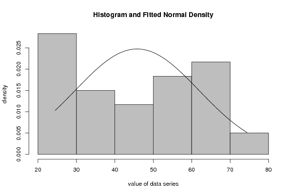
| Title produced by software | Maximum-likelihood Fitting - Normal Distribution | ||||||||||||||||||||||||||||||||||||||
| Date of computation | Sun, 23 Nov 2008 08:59:00 -0700 | ||||||||||||||||||||||||||||||||||||||
| Cite this page as follows | Statistical Computations at FreeStatistics.org, Office for Research Development and Education, URL https://freestatistics.org/blog/index.php?v=date/2008/Nov/23/t12274560019d1kfvdiq8zudlq.htm/, Retrieved Sun, 13 Jul 2025 08:00:53 +0000 | ||||||||||||||||||||||||||||||||||||||
| Statistical Computations at FreeStatistics.org, Office for Research Development and Education, URL https://freestatistics.org/blog/index.php?pk=25293, Retrieved Sun, 13 Jul 2025 08:00:53 +0000 | |||||||||||||||||||||||||||||||||||||||
| QR Codes: | |||||||||||||||||||||||||||||||||||||||
|
| |||||||||||||||||||||||||||||||||||||||
| Original text written by user: | |||||||||||||||||||||||||||||||||||||||
| IsPrivate? | No (this computation is public) | ||||||||||||||||||||||||||||||||||||||
| User-defined keywords | |||||||||||||||||||||||||||||||||||||||
| Estimated Impact | 255 | ||||||||||||||||||||||||||||||||||||||
Tree of Dependent Computations | |||||||||||||||||||||||||||||||||||||||
| Family? (F = Feedback message, R = changed R code, M = changed R Module, P = changed Parameters, D = changed Data) | |||||||||||||||||||||||||||||||||||||||
| F [Box-Cox Linearity Plot] [Q3] [2008-11-11 16:15:27] [299afd6311e4c20059ea2f05c8dd029d] F D [Box-Cox Linearity Plot] [Q4] [2008-11-11 16:18:23] [299afd6311e4c20059ea2f05c8dd029d] F RMPD [Maximum-likelihood Fitting - Normal Distribution] [Q5] [2008-11-11 16:26:11] [299afd6311e4c20059ea2f05c8dd029d] - D [Maximum-likelihood Fitting - Normal Distribution] [Verbetering Q5] [2008-11-23 15:59:00] [5e2b1e7aa808f9f0d23fd35605d4968f] [Current] | |||||||||||||||||||||||||||||||||||||||
| Feedback Forum | |||||||||||||||||||||||||||||||||||||||
Post a new message | |||||||||||||||||||||||||||||||||||||||
Dataset | |||||||||||||||||||||||||||||||||||||||
| Dataseries X: | |||||||||||||||||||||||||||||||||||||||
24,67 25,59 26,09 28,37 27,34 24,46 27,46 30,23 32,33 29,87 24,87 25,48 27,28 28,24 29,58 26,95 29,08 28,76 29,59 30,7 30,52 32,67 33,19 37,13 35,54 37,75 41,84 42,94 49,14 44,61 40,22 44,23 45,85 53,38 53,26 51,8 55,3 57,81 63,96 63,77 59,15 56,12 57,42 63,52 61,71 63,01 68,18 72,03 69,75 74,41 74,33 64,24 60,03 59,44 62,5 55,04 58,34 61,92 67,65 67,68 | |||||||||||||||||||||||||||||||||||||||
Tables (Output of Computation) | |||||||||||||||||||||||||||||||||||||||
| |||||||||||||||||||||||||||||||||||||||
Figures (Output of Computation) | |||||||||||||||||||||||||||||||||||||||
Input Parameters & R Code | |||||||||||||||||||||||||||||||||||||||
| Parameters (Session): | |||||||||||||||||||||||||||||||||||||||
| par1 = 8 ; par2 = 0 ; | |||||||||||||||||||||||||||||||||||||||
| Parameters (R input): | |||||||||||||||||||||||||||||||||||||||
| par1 = 8 ; par2 = 0 ; | |||||||||||||||||||||||||||||||||||||||
| R code (references can be found in the software module): | |||||||||||||||||||||||||||||||||||||||
library(MASS) | |||||||||||||||||||||||||||||||||||||||