Free Statistics
of Irreproducible Research!
Description of Statistical Computation | |||||||||||||||||||||||||||||||||||||||||||||||||||||
|---|---|---|---|---|---|---|---|---|---|---|---|---|---|---|---|---|---|---|---|---|---|---|---|---|---|---|---|---|---|---|---|---|---|---|---|---|---|---|---|---|---|---|---|---|---|---|---|---|---|---|---|---|---|
| Author's title | |||||||||||||||||||||||||||||||||||||||||||||||||||||
| Author | *The author of this computation has been verified* | ||||||||||||||||||||||||||||||||||||||||||||||||||||
| R Software Module | rwasp_edauni.wasp | ||||||||||||||||||||||||||||||||||||||||||||||||||||
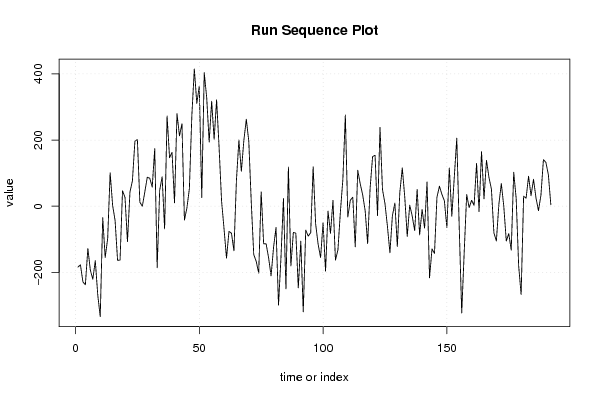
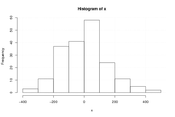
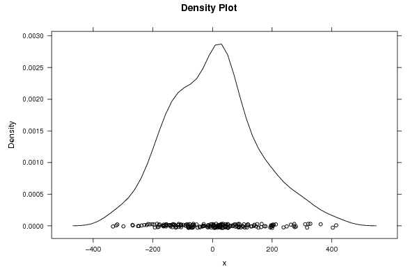
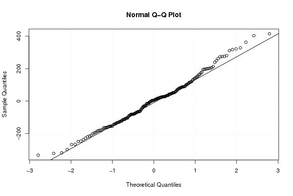
| Title produced by software | Univariate Explorative Data Analysis | ||||||||||||||||||||||||||||||||||||||||||||||||||||
| Date of computation | Wed, 19 Nov 2008 07:06:25 -0700 | ||||||||||||||||||||||||||||||||||||||||||||||||||||
| Cite this page as follows | Statistical Computations at FreeStatistics.org, Office for Research Development and Education, URL https://freestatistics.org/blog/index.php?v=date/2008/Nov/19/t1227103620q54x9nc6wvfta50.htm/, Retrieved Sat, 12 Jul 2025 01:23:45 +0000 | ||||||||||||||||||||||||||||||||||||||||||||||||||||
| Statistical Computations at FreeStatistics.org, Office for Research Development and Education, URL https://freestatistics.org/blog/index.php?pk=25034, Retrieved Sat, 12 Jul 2025 01:23:45 +0000 | |||||||||||||||||||||||||||||||||||||||||||||||||||||
| QR Codes: | |||||||||||||||||||||||||||||||||||||||||||||||||||||
|
| |||||||||||||||||||||||||||||||||||||||||||||||||||||
| Original text written by user: | |||||||||||||||||||||||||||||||||||||||||||||||||||||
| IsPrivate? | No (this computation is public) | ||||||||||||||||||||||||||||||||||||||||||||||||||||
| User-defined keywords | |||||||||||||||||||||||||||||||||||||||||||||||||||||
| Estimated Impact | 320 | ||||||||||||||||||||||||||||||||||||||||||||||||||||
Tree of Dependent Computations | |||||||||||||||||||||||||||||||||||||||||||||||||||||
| Family? (F = Feedback message, R = changed R code, M = changed R Module, P = changed Parameters, D = changed Data) | |||||||||||||||||||||||||||||||||||||||||||||||||||||
| F [Multiple Regression] [Taak 6 - Q1 (2)] [2008-11-16 10:42:33] [46c5a5fbda57fdfa1d4ef48658f82a0c] F RMPD [Univariate Explorative Data Analysis] [Taak 6 Q 2] [2008-11-19 14:06:25] [bda7fba231d49184c6a1b627868bbb81] [Current] F PD [Univariate Explorative Data Analysis] [Q2 task 6] [2008-11-20 17:26:46] [8eb83367d7ce233bbf617141d324189b] F PD [Univariate Explorative Data Analysis] [Seatbelt Law Q2] [2008-11-23 13:04:24] [3548296885df7a66ea8efc200c4aca50] - [Univariate Explorative Data Analysis] [Seatbelt Law Q2] [2008-11-23 12:29:32] [3548296885df7a66ea8efc200c4aca50] - PD [Univariate Explorative Data Analysis] [Q2 Seatbelt law] [2008-11-30 13:42:21] [7d3039e6253bb5fb3b26df1537d500b4] | |||||||||||||||||||||||||||||||||||||||||||||||||||||
| Feedback Forum | |||||||||||||||||||||||||||||||||||||||||||||||||||||
Post a new message | |||||||||||||||||||||||||||||||||||||||||||||||||||||
Dataset | |||||||||||||||||||||||||||||||||||||||||||||||||||||
| Dataseries X: | |||||||||||||||||||||||||||||||||||||||||||||||||||||
-183,9235445 -177,0726091 -228,6351091 -237,4476091 -127,7601091 -193,0101091 -220,6351091 -164,5101091 -268,3226091 -333,6976091 -34,26010911 -154,8851091 -97,74528053 101,1056549 2,543154874 -43,26934513 -163,5818451 -162,8318451 46,54315487 26,66815487 -107,1443451 42,48065487 76,91815487 196,2931549 201,4329835 12,28391886 -0,278581137 42,90891886 87,59641886 84,34641886 57,72141886 173,8464189 -185,9660811 47,65891886 89,09641886 -68,52858114 272,6112475 146,4621829 162,8996829 10,08718285 279,7746829 212,5246829 248,8996829 -41,97531715 -5,787817149 52,83718285 274,2746829 414,6496829 310,7895114 362,6404468 26,07794684 403,2654468 327,9529468 193,7029468 317,0779468 202,2029468 321,3904468 178,0154468 16,45294684 -68,17205316 -157,0322246 -76,18128917 -81,74378917 -134,5562892 77,13121083 199,8812108 105,2562108 198,3812108 262,5687108 196,1937108 11,63121083 -145,9937892 -166,8539606 -202,0030252 43,43447482 -113,3780252 -113,6905252 -155,9405252 -210,5655252 -124,4405252 -64,25302518 -298,6280252 -154,1905252 23,18447482 -249,6756966 118,1752388 -180,3872612 -79,19976119 -81,51226119 -246,7622612 -105,3872612 -319,2622612 -72,07476119 -90,44976119 -80,01226119 119,3627388 -53,49743261 -114,6464972 -155,2089972 -50,02149721 -196,3339972 -14,58399721 -82,20899721 17,91600279 -162,8964972 -132,2714972 -16,83399721 81,54100279 275,6808314 -32,46823322 17,96926678 27,15676678 -123,1557332 108,5942668 67,96926678 34,09426678 -13,71823322 -113,0932332 54,34426678 149,7192668 153,8590954 -28,28996923 238,1475308 50,33503077 8,022530771 -61,22746923 -140,8524692 -28,72746923 9,460030771 -121,9149692 41,52253077 115,8975308 27,03735936 -91,11170524 3,325794759 -29,48670524 -73,79920524 50,95079476 -86,67420524 -9,54920524 -66,36170524 73,26329476 -216,2992052 -128,9242052 -142,7843767 27,06655875 60,50405875 35,69155875 16,37905875 -64,87094125 115,5040587 -30,37094125 87,81655875 205,4415587 -64,12094125 -322,7459413 -139,6061127 35,24482274 -4,317677263 17,86982274 2,557322737 129,3073227 -16,31767726 164,8073227 21,99482274 138,6198227 87,05732274 51,43232274 -80,42784867 -105,1918797 5,245620328 68,43312033 -0,879379672 -105,1293797 -82,75437967 -132,6293797 102,5581203 23,18312033 -180,3793797 -267,0043797 30,13544892 23,98638432 90,42388432 31,61138432 81,29888432 25,04888432 -13,57611568 33,54888432 140,7363843 132,3613843 94,79888432 4,173884316 | |||||||||||||||||||||||||||||||||||||||||||||||||||||
Tables (Output of Computation) | |||||||||||||||||||||||||||||||||||||||||||||||||||||
| |||||||||||||||||||||||||||||||||||||||||||||||||||||
Figures (Output of Computation) | |||||||||||||||||||||||||||||||||||||||||||||||||||||
Input Parameters & R Code | |||||||||||||||||||||||||||||||||||||||||||||||||||||
| Parameters (Session): | |||||||||||||||||||||||||||||||||||||||||||||||||||||
| par1 = 0 ; par2 = 0 ; | |||||||||||||||||||||||||||||||||||||||||||||||||||||
| Parameters (R input): | |||||||||||||||||||||||||||||||||||||||||||||||||||||
| par1 = 0 ; par2 = 0 ; | |||||||||||||||||||||||||||||||||||||||||||||||||||||
| R code (references can be found in the software module): | |||||||||||||||||||||||||||||||||||||||||||||||||||||
par1 <- as.numeric(par1) | |||||||||||||||||||||||||||||||||||||||||||||||||||||