Repository of Reproducible Computations

Free Statistics

of Irreproducible Research!

Author's title

Author

*Unverified author*

R Software Module

rwasp_fitdistrnorm.wasp

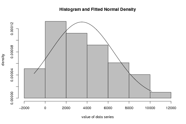
Title produced by software

Maximum-likelihood Fitting - Normal Distribution

Date of computation

Thu, 13 Nov 2008 15:37:20 -0700

Cite this page as follows

Statistical Computations at FreeStatistics.org, Office for Research Development and Education, URL https://freestatistics.org/blog/index.php?v=date/2008/Nov/13/t1226615867p1s5tkexy3rt726.htm/, Retrieved Tue, 28 May 2024 12:26:31 +0000

Statistical Computations at FreeStatistics.org, Office for Research Development and Education, URL https://freestatistics.org/blog/index.php?pk=24873, Retrieved Tue, 28 May 2024 12:26:31 +0000

QR Codes:

Paste this QR Code to cite your computation.

Original text written by user:

IsPrivate?

No (this computation is public)

User-defined keywords

Estimated Impact

190

Family? (F = Feedback message, R = changed R code, M = changed R Module, P = changed Parameters, D = changed Data)

-     [Bivariate Kernel Density Estimation] [Bel20 en Downjones] [2008-11-12 17:23:23] [74be16979710d4c4e7c6647856088456]
F RMPD  [Maximum-likelihood Fitting - Normal Distribution] [kelly] [2008-11-12 17:58:06] [74be16979710d4c4e7c6647856088456]
F    D      [Maximum-likelihood Fitting - Normal Distribution] [normality] [2008-11-13 22:37:20] [d41d8cd98f00b204e9800998ecf8427e] [Current]

Feedback Forum

2008-11-16 11:40:54 [Nicolaj Wuyts] [reply] 
De gegevens zijn niet normaal verdeeld. De mediaan ligt rond de 3500 terwijl die bij een normaalverdeling rond de 7000 zou moeten liggen. Ook zien we dat de grafiek een staart heeft naar de linkerkant toe. Dit wijst op een linksscheve verdeling.
2008-11-23 14:04:22 [c97d2ae59c98cf77a04815c1edffab5a] [reply] 
de student heeft de figuren juist geproduceerd, maar er is geen conclusie gevormd. Allereerst moeten we vermelden dat De tabel geeft het geschatte gemiddelde (3498) en standaarddeviatie (3030) weer. De lijn op de figuur vormt de geschatte normaalverdeling die het dichtst bij het histogram aanleunt. We kunnen hier stellen dat de verdeling niet normaal verdeeld is, maar linksscheef verdeeld.Bij een normaalverdeling zou het gemiddelde ongeveer in het midden van het histogram liggen (4000), maar doordat de data linksscheef zijn verdeeld (meeste data liggen rechts=> hoogste dichtheid) zal het gemiddelde dus eerder aan de rechtse kant liggen, wat dus klopt: 3498<4000
2008-11-24 10:53:36 [Julian De Ruyter] [reply] 
Juiste histogram, geen conclusie. 
mean = 3498.93877551020 
standard deviation = 3030.75887585906 
 
De gegevens zijn niet normaalverdeeld. Anders zou het gemiddelde rond 4000 moeten liggen(meer naar rechts). De staart van de verdeling van de gegevens wijst op een linksscheve verdeling. 
2008-11-24 20:08:01 [Liese Drijkoningen] [reply] 
De juiste grafiek werd geproduceerd. We kunnen hier uit afleiden dat deze variabele relatief normaal verdeeld is. Dit kunnen we afleiden uit het histogram met een normaalverdeling.
2008-11-24 21:10:34 [Jonas Scheltjens] [reply] 
Q5: De student geeft hier geen besluit. Door de methode “Maximum-likelihood Normal Distribution Fitting” te gebruiken kunnen we kijken of de gegevens al dan niet normaal verdeeld zijn. De grafiek bevat de lijn die de normaalverdeling tracht na te bootsen en een histogram. In deze opgave (met deze gegevens) is er de normaalverdeling niet echt merkbaar. De histogram laat ons zien dat er een rechtsscheve verdeling is en de lijn is volgt ook het patroon van een normaalverdeling niet.

Post a new message

Dataseries X:

Download CSV

Histogram

Boxplots

Summary of computational transaction
Raw Input	view raw input (R code)
Raw Output	view raw output of R engine
Computing time	1 seconds
R Server	'George Udny Yule' @ 72.249.76.132

\begin{tabular}{lllllllll}
\hline
Summary of computational transaction \tabularnewline
Raw Input & view raw input (R code)  \tabularnewline
Raw Output & view raw output of R engine  \tabularnewline
Computing time & 1 seconds \tabularnewline
R Server & 'George Udny Yule' @ 72.249.76.132 \tabularnewline
\hline
\end{tabular}
%Source: https://freestatistics.org/blog/index.php?pk=24873&T=0

[TABLE]
[ROW][C]Summary of computational transaction[/C][/ROW]
[ROW][C]Raw Input[/C][C]view raw input (R code) [/C][/ROW]
[ROW][C]Raw Output[/C][C]view raw output of R engine [/C][/ROW]
[ROW][C]Computing time[/C][C]1 seconds[/C][/ROW]
[ROW][C]R Server[/C][C]'George Udny Yule' @ 72.249.76.132[/C][/ROW]
[/TABLE]
Source: https://freestatistics.org/blog/index.php?pk=24873&T=0

Globally Unique Identifier (entire table): ba.freestatistics.org/blog/index.php?pk=24873&T=0

As an alternative you can also use a QR Code:

The GUIDs for individual cells are displayed in the table below:

Summary of computational transaction
Raw Input	view raw input (R code)
Raw Output	view raw output of R engine
Computing time	1 seconds
R Server	'George Udny Yule' @ 72.249.76.132

Parameter	Estimated Value	Standard Deviation
mean	3498.93877551020	432.965553694152
standard deviation	3030.75887585906	306.152879037323

\begin{tabular}{lllllllll}
\hline
Parameter & Estimated Value & Standard Deviation \tabularnewline
mean & 3498.93877551020 & 432.965553694152 \tabularnewline
standard deviation & 3030.75887585906 & 306.152879037323 \tabularnewline
\hline
\end{tabular}
%Source: https://freestatistics.org/blog/index.php?pk=24873&T=1

[TABLE]
[ROW][C]Parameter[/C][C]Estimated Value[/C][C]Standard Deviation[/C][/ROW]
[ROW][C]mean[/C][C]3498.93877551020[/C][C]432.965553694152[/C][/ROW]
[ROW][C]standard deviation[/C][C]3030.75887585906[/C][C]306.152879037323[/C][/ROW]
[/TABLE]
Source: https://freestatistics.org/blog/index.php?pk=24873&T=1

Globally Unique Identifier (entire table): ba.freestatistics.org/blog/index.php?pk=24873&T=1

As an alternative you can also use a QR Code:

The GUIDs for individual cells are displayed in the table below:

Parameter	Estimated Value	Standard Deviation
mean	3498.93877551020	432.965553694152
standard deviation	3030.75887585906	306.152879037323

Figure 1

PNG link

Postscript link

PDF link

Parameters (Session):

par1 = 8 ; par2 = 0 ;

Parameters (R input):

par1 = 8 ; par2 = 0 ;

R code (references can be found in the software module):

library(MASS)
par1 <- as.numeric(par1)
if (par2 == '0') par2 = 'Sturges' else par2 <- as.numeric(par2)
x <- as.ts(x) #otherwise the fitdistr function does not work properly
r <- fitdistr(x,'normal')
r
bitmap(file='test1.png')
myhist<-hist(x,col=par1,breaks=par2,main=main,ylab=ylab,xlab=xlab,freq=F)
curve(1/(r$estimate[2]*sqrt(2*pi))*exp(-1/2*((x-r$estimate[1])/r$estimate[2])^2),min(x),max(x),add=T)
dev.off()
load(file='createtable')
a<-table.start()
a<-table.row.start(a)
a<-table.element(a,'Parameter',1,TRUE)
a<-table.element(a,'Estimated Value',1,TRUE)
a<-table.element(a,'Standard Deviation',1,TRUE)
a<-table.row.end(a)
a<-table.row.start(a)
a<-table.element(a,'mean',header=TRUE)
a<-table.element(a,r$estimate[1])
a<-table.element(a,r$sd[1])
a<-table.row.end(a)
a<-table.row.start(a)
a<-table.element(a,'standard deviation',header=TRUE)
a<-table.element(a,r$estimate[2])
a<-table.element(a,r$sd[2])
a<-table.row.end(a)
a<-table.end(a)
table.save(a,file='mytable.tab')

Free Statistics

Description of Statistical Computation

Tree of Dependent Computations

Dataset

Tables (Output of Computation)

Figures (Output of Computation)

Input Parameters & R Code