Free Statistics
of Irreproducible Research!
Description of Statistical Computation | |||||||||||||||||||||||||||||||||||||
|---|---|---|---|---|---|---|---|---|---|---|---|---|---|---|---|---|---|---|---|---|---|---|---|---|---|---|---|---|---|---|---|---|---|---|---|---|---|
| Author's title | |||||||||||||||||||||||||||||||||||||
| Author | *Unverified author* | ||||||||||||||||||||||||||||||||||||
| R Software Module | rwasp_boxcoxnorm.wasp | ||||||||||||||||||||||||||||||||||||
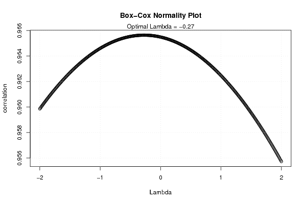
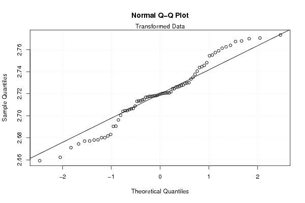
| Title produced by software | Box-Cox Normality Plot | ||||||||||||||||||||||||||||||||||||
| Date of computation | Thu, 13 Nov 2008 13:20:28 -0700 | ||||||||||||||||||||||||||||||||||||
| Cite this page as follows | Statistical Computations at FreeStatistics.org, Office for Research Development and Education, URL https://freestatistics.org/blog/index.php?v=date/2008/Nov/13/t1226607709ywk9dbrb0ch17mp.htm/, Retrieved Sun, 19 May 2024 10:46:40 +0000 | ||||||||||||||||||||||||||||||||||||
| Statistical Computations at FreeStatistics.org, Office for Research Development and Education, URL https://freestatistics.org/blog/index.php?pk=24822, Retrieved Sun, 19 May 2024 10:46:40 +0000 | |||||||||||||||||||||||||||||||||||||
| QR Codes: | |||||||||||||||||||||||||||||||||||||
|
| |||||||||||||||||||||||||||||||||||||
| Original text written by user: | |||||||||||||||||||||||||||||||||||||
| IsPrivate? | No (this computation is public) | ||||||||||||||||||||||||||||||||||||
| User-defined keywords | |||||||||||||||||||||||||||||||||||||
| Estimated Impact | 148 | ||||||||||||||||||||||||||||||||||||
Tree of Dependent Computations | |||||||||||||||||||||||||||||||||||||
| Family? (F = Feedback message, R = changed R code, M = changed R Module, P = changed Parameters, D = changed Data) | |||||||||||||||||||||||||||||||||||||
| F [Box-Cox Linearity Plot] [question 3 box-co...] [2008-11-12 15:13:33] [31c9f333c18b3396ccf9d2485dd39c8a] F RM D [Box-Cox Normality Plot] [Vincent Dolhain T...] [2008-11-13 20:20:28] [dcb9dbe132bac62365bf3d43fe342148] [Current] F RMPD [Maximum-likelihood Fitting - Normal Distribution] [Taak 2 Part 1 Oef5] [2008-11-13 20:29:43] [17bef6922a2795858ae28bf8ba596537] | |||||||||||||||||||||||||||||||||||||
| Feedback Forum | |||||||||||||||||||||||||||||||||||||
Post a new message | |||||||||||||||||||||||||||||||||||||
Dataset | |||||||||||||||||||||||||||||||||||||
| Dataseries X: | |||||||||||||||||||||||||||||||||||||
109,86 108,68 113,38 117,12 116,23 114,75 115,81 115,86 117,8 117,11 116,31 118,38 121,57 121,65 124,2 126,12 128,6 128,16 130,12 135,83 138,05 134,99 132,38 128,94 128,12 127,84 132,43 134,13 134,78 133,13 129,08 134,48 132,86 134,08 134,54 134,51 135,97 136,09 139,14 135,63 136,55 138,83 138,84 135,37 132,22 134,75 135,98 136,06 138,05 139,59 140,58 139,81 140,77 140,96 143,59 142,7 145,11 146,7 148,53 148,99 149,65 151,11 154,82 156,56 157,6 155,24 160,68 163,22 164,55 166,76 159,05 159,82 164,95 162,89 | |||||||||||||||||||||||||||||||||||||
Tables (Output of Computation) | |||||||||||||||||||||||||||||||||||||
| |||||||||||||||||||||||||||||||||||||
Figures (Output of Computation) | |||||||||||||||||||||||||||||||||||||
Input Parameters & R Code | |||||||||||||||||||||||||||||||||||||
| Parameters (Session): | |||||||||||||||||||||||||||||||||||||
| Parameters (R input): | |||||||||||||||||||||||||||||||||||||
| R code (references can be found in the software module): | |||||||||||||||||||||||||||||||||||||
n <- length(x) | |||||||||||||||||||||||||||||||||||||