Repository of Reproducible Computations

Free Statistics

of Irreproducible Research!

Author's title

Author

*The author of this computation has been verified*

R Software Module

rwasp_bidensity.wasp

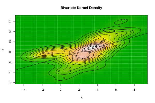
Title produced by software

Bivariate Kernel Density Estimation

Date of computation

Thu, 13 Nov 2008 09:17:37 -0700

Cite this page as follows

Statistical Computations at FreeStatistics.org, Office for Research Development and Education, URL https://freestatistics.org/blog/index.php?v=date/2008/Nov/13/t12265931260b4u4zl8xbcqx0m.htm/, Retrieved Sun, 19 May 2024 10:42:36 +0000

Statistical Computations at FreeStatistics.org, Office for Research Development and Education, URL https://freestatistics.org/blog/index.php?pk=24672, Retrieved Sun, 19 May 2024 10:42:36 +0000

QR Codes:

Paste this QR Code to cite your computation.

Original text written by user:

IsPrivate?

No (this computation is public)

User-defined keywords

Estimated Impact

148

Family? (F = Feedback message, R = changed R code, M = changed R Module, P = changed Parameters, D = changed Data)

F       [Bivariate Kernel Density Estimation] [Q1] [2008-11-13 16:17:37] [8e1dd6a8d7300d49f515697199ea9e73] [Current]

Feedback Forum

2008-11-14 15:42:51 [Annemiek Hoofman] [reply] 
Ik denk dat alle observaties binnen de hoogtelijnen liggen, maar hier ben ik niet zeker van.
2008-11-19 19:48:07 [] [reply] 
Via de Bivariate Density plot wordt er een verband gezocht tussen 2 variabelen. Deze worden weergegeven in een vorm van een scatterplot met een regressielijn (lijn die alle punten het beste benadert) en met hoogtelijnen (i.v.m de dichtheid, geeft de kans weer dat men op bepaald niveau zit en deze kans is  bij de ene hoogtelijn groter dan bij de andere). Hoe meer de punten op ongeveer dezelfde lijn liggen, hoe hoger de correlatie. Hierbij kunnen we zeggen dat de correlatie niet zo heel sterk is. Dit is dan ook af te leiden uit de tabel (0,58). 
2008-11-24 22:31:33 [Erik Geysen] [reply] 
De regressielijn is de best mogelijke functie die de puntenwolk zo dicht mogelijk benadert.  
Het voordeel van de Bivariate Density Plot zien we of er een wetmatigheid bestaat voor een bepaalde periode.  
Als de hoogtelijnen hebben een  cirkelvorm hebben bestaat er geen correlatie. Hebben ze een ellipsvorm dan kunnen we wel spreken van een verband.Hoe meer punten op de hoogtelijnen, hoe sterker de correlatie. In dit voorbeeld is er geen sterke correlatie. Dit concludeer ik aan de hand van het getal 0,58 dat we in de tabel terug vinden.   
 

Post a new message

Dataseries X:

Download CSV

Histogram

Boxplots

-0,2
1,0
0,4
1,0
1,7
3,1
3,3
3,1
3,5
6,0
5,7
4,7
4,2
3,6
4,4
2,5
-0,6
-1,9
-1,9
0,7
-0,9
-1,7
-3,1
-2,1
0,2
1,2
3,8
4,0
6,6
5,3
7,6
4,7
6,6
4,4
4,6
6,0
4,8
4,0
2,7
3,0
4,1
4,0
2,7
2,6
3,1
4,4
3,0
2,0
1,3
1,5
1,3
3,2
1,8
3,3
1,0
2,4
0,4
-1,1

Dataseries Y:

Download CSV

Histogram

4,3
4,2
2,9
4,9
7,2
8,7
9,1
8,9
9,0
11,6
9,6
9,1
9,2
10,8
11,0
8,5
6,5
7,2
7,8
8,7
7,8
7,5
7,7
7,5
8,3
7,9
10,4
11,5
14,0
11,9
11,9
10,3
11,3
9,9
8,9
9,2
8,8
6,7
7,1
6,6
7,2
5,0
5,3
6,3
8,0
7,6
7,0
6,9
6,8
7,5
6,4
8,0
6,4
9,5
7,6
9,1
8,2
8,5

Summary of computational transaction
Raw Input	view raw input (R code)
Raw Output	view raw output of R engine
Computing time	1 seconds
R Server	'Gwilym Jenkins' @ 72.249.127.135

\begin{tabular}{lllllllll}
\hline
Summary of computational transaction \tabularnewline
Raw Input & view raw input (R code)  \tabularnewline
Raw Output & view raw output of R engine  \tabularnewline
Computing time & 1 seconds \tabularnewline
R Server & 'Gwilym Jenkins' @ 72.249.127.135 \tabularnewline
\hline
\end{tabular}
%Source: https://freestatistics.org/blog/index.php?pk=24672&T=0

[TABLE]
[ROW][C]Summary of computational transaction[/C][/ROW]
[ROW][C]Raw Input[/C][C]view raw input (R code) [/C][/ROW]
[ROW][C]Raw Output[/C][C]view raw output of R engine [/C][/ROW]
[ROW][C]Computing time[/C][C]1 seconds[/C][/ROW]
[ROW][C]R Server[/C][C]'Gwilym Jenkins' @ 72.249.127.135[/C][/ROW]
[/TABLE]
Source: https://freestatistics.org/blog/index.php?pk=24672&T=0

Globally Unique Identifier (entire table): ba.freestatistics.org/blog/index.php?pk=24672&T=0

As an alternative you can also use a QR Code:

The GUIDs for individual cells are displayed in the table below:

Summary of computational transaction
Raw Input	view raw input (R code)
Raw Output	view raw output of R engine
Computing time	1 seconds
R Server	'Gwilym Jenkins' @ 72.249.127.135

Bandwidth
x axis	1.11800427166590
y axis	0.713543038197552
Correlation
correlation used in KDE	0.580647425021013
correlation(x,y)	0.580647425021013

\begin{tabular}{lllllllll}
\hline
Bandwidth \tabularnewline
x axis & 1.11800427166590 \tabularnewline
y axis & 0.713543038197552 \tabularnewline
Correlation \tabularnewline
correlation used in KDE & 0.580647425021013 \tabularnewline
correlation(x,y) & 0.580647425021013 \tabularnewline
\hline
\end{tabular}
%Source: https://freestatistics.org/blog/index.php?pk=24672&T=1

[TABLE]
[ROW][C]Bandwidth[/C][/ROW]
[ROW][C]x axis[/C][C]1.11800427166590[/C][/ROW]
[ROW][C]y axis[/C][C]0.713543038197552[/C][/ROW]
[ROW][C]Correlation[/C][/ROW]
[ROW][C]correlation used in KDE[/C][C]0.580647425021013[/C][/ROW]
[ROW][C]correlation(x,y)[/C][C]0.580647425021013[/C][/ROW]
[/TABLE]
Source: https://freestatistics.org/blog/index.php?pk=24672&T=1

Globally Unique Identifier (entire table): ba.freestatistics.org/blog/index.php?pk=24672&T=1

As an alternative you can also use a QR Code:

The GUIDs for individual cells are displayed in the table below:

Bandwidth
x axis	1.11800427166590
y axis	0.713543038197552
Correlation
correlation used in KDE	0.580647425021013
correlation(x,y)	0.580647425021013

Figure 1

PNG link

Postscript link

PDF link

Parameters (Session):

par1 = 50 ; par2 = 50 ; par3 = 0 ; par4 = 0 ; par5 = 0 ; par6 = Y ; par7 = Y ;

Parameters (R input):

par1 = 50 ; par2 = 50 ; par3 = 0 ; par4 = 0 ; par5 = 0 ; par6 = Y ; par7 = Y ;

R code (references can be found in the software module):

par1 <- as(par1,'numeric')
par2 <- as(par2,'numeric')
par3 <- as(par3,'numeric')
par4 <- as(par4,'numeric')
par5 <- as(par5,'numeric')
library('GenKern')
if (par3==0) par3 <- dpik(x)
if (par4==0) par4 <- dpik(y)
if (par5==0) par5 <- cor(x,y)
if (par1 > 500) par1 <- 500
if (par2 > 500) par2 <- 500
bitmap(file='bidensity.png')
op <- KernSur(x,y, xgridsize=par1, ygridsize=par2, correlation=par5, xbandwidth=par3, ybandwidth=par4)
image(op$xords, op$yords, op$zden, col=terrain.colors(100), axes=TRUE,main=main,xlab=xlab,ylab=ylab)
if (par6=='Y') contour(op$xords, op$yords, op$zden, add=TRUE)
if (par7=='Y') points(x,y)
(r<-lm(y ~ x))
abline(r)
box()
dev.off()
load(file='createtable')
a<-table.start()
a<-table.row.start(a)
a<-table.element(a,'Bandwidth',2,TRUE)
a<-table.row.end(a)
a<-table.row.start(a)
a<-table.element(a,'x axis',header=TRUE)
a<-table.element(a,par3)
a<-table.row.end(a)
a<-table.row.start(a)
a<-table.element(a,'y axis',header=TRUE)
a<-table.element(a,par4)
a<-table.row.end(a)
a<-table.row.start(a)
a<-table.element(a,'Correlation',2,TRUE)
a<-table.row.end(a)
a<-table.row.start(a)
a<-table.element(a,'correlation used in KDE',header=TRUE)
a<-table.element(a,par5)
a<-table.row.end(a)
a<-table.row.start(a)
a<-table.element(a,'correlation(x,y)',header=TRUE)
a<-table.element(a,cor(x,y))
a<-table.row.end(a)
a<-table.end(a)
table.save(a,file='mytable.tab')

Free Statistics

Description of Statistical Computation

Tree of Dependent Computations

Dataset

Tables (Output of Computation)

Figures (Output of Computation)

Input Parameters & R Code