Free Statistics
of Irreproducible Research!
Description of Statistical Computation | |||||||||||||||||||||||||||||||||||||||
|---|---|---|---|---|---|---|---|---|---|---|---|---|---|---|---|---|---|---|---|---|---|---|---|---|---|---|---|---|---|---|---|---|---|---|---|---|---|---|---|
| Author's title | |||||||||||||||||||||||||||||||||||||||
| Author | *The author of this computation has been verified* | ||||||||||||||||||||||||||||||||||||||
| R Software Module | rwasp_fitdistrnorm.wasp | ||||||||||||||||||||||||||||||||||||||
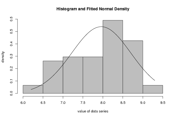
| Title produced by software | Maximum-likelihood Fitting - Normal Distribution | ||||||||||||||||||||||||||||||||||||||
| Date of computation | Thu, 13 Nov 2008 03:44:33 -0700 | ||||||||||||||||||||||||||||||||||||||
| Cite this page as follows | Statistical Computations at FreeStatistics.org, Office for Research Development and Education, URL https://freestatistics.org/blog/index.php?v=date/2008/Nov/13/t12265731365z9nj4qbr9qv7n6.htm/, Retrieved Sun, 19 May 2024 10:42:28 +0000 | ||||||||||||||||||||||||||||||||||||||
| Statistical Computations at FreeStatistics.org, Office for Research Development and Education, URL https://freestatistics.org/blog/index.php?pk=24559, Retrieved Sun, 19 May 2024 10:42:28 +0000 | |||||||||||||||||||||||||||||||||||||||
| QR Codes: | |||||||||||||||||||||||||||||||||||||||
|
| |||||||||||||||||||||||||||||||||||||||
| Original text written by user: | |||||||||||||||||||||||||||||||||||||||
| IsPrivate? | No (this computation is public) | ||||||||||||||||||||||||||||||||||||||
| User-defined keywords | Normal ML Fit | ||||||||||||||||||||||||||||||||||||||
| Estimated Impact | 182 | ||||||||||||||||||||||||||||||||||||||
Tree of Dependent Computations | |||||||||||||||||||||||||||||||||||||||
| Family? (F = Feedback message, R = changed R code, M = changed R Module, P = changed Parameters, D = changed Data) | |||||||||||||||||||||||||||||||||||||||
| F [Maximum-likelihood Fitting - Normal Distribution] [workshop 2 Q5 Nor...] [2008-11-13 10:44:33] [74c7506a1ea162af3aa8be25bcd05d28] [Current] F R D [Maximum-likelihood Fitting - Normal Distribution] [Normal distribution] [2008-11-13 19:18:39] [3ffd109c9e040b1ae7e5dbe576d4698c] - RMPD [Notched Boxplots] [notched boxplot] [2008-12-10 18:45:46] [3ffd109c9e040b1ae7e5dbe576d4698c] - [Notched Boxplots] [Notched Boxplot] [2008-12-17 09:34:11] [3ffd109c9e040b1ae7e5dbe576d4698c] - D [Notched Boxplots] [notched boxplot] [2008-12-20 11:57:36] [3ffd109c9e040b1ae7e5dbe576d4698c] - D [Notched Boxplots] [notched boxplot] [2008-12-20 11:59:33] [3ffd109c9e040b1ae7e5dbe576d4698c] - D [Notched Boxplots] [notched boxplot] [2008-12-20 12:02:04] [3ffd109c9e040b1ae7e5dbe576d4698c] - [Notched Boxplots] [notched boxplots] [2008-12-24 11:50:45] [3f66c6f083b1153972739491b89fa2dd] - RMPD [Mean Plot] [mean plot] [2008-12-10 18:47:53] [3ffd109c9e040b1ae7e5dbe576d4698c] - [Mean Plot] [mean plot] [2008-12-18 18:13:03] [3ffd109c9e040b1ae7e5dbe576d4698c] - [Mean Plot] [Mean plot] [2008-12-24 11:53:26] [3f66c6f083b1153972739491b89fa2dd] | |||||||||||||||||||||||||||||||||||||||
| Feedback Forum | |||||||||||||||||||||||||||||||||||||||
Post a new message | |||||||||||||||||||||||||||||||||||||||
Dataset | |||||||||||||||||||||||||||||||||||||||
| Dataseries X: | |||||||||||||||||||||||||||||||||||||||
8,4 8,4 8,4 8,6 8,9 8,8 8,3 7,5 7,2 7,5 8,8 9,3 9,3 8,7 8,2 8,3 8,5 8,6 8,6 8,2 8,1 8 8,6 8,7 8,8 8,5 8,4 8,5 8,7 8,7 8,6 8,5 8,3 8,1 8,2 8,1 8,1 7,9 7,9 7,9 8 8 7,9 8 7,7 7,2 7,5 7,3 7 7 7 7,2 7,3 7,1 6,8 6,6 6,2 6,2 6,8 6,9 6,8 | |||||||||||||||||||||||||||||||||||||||
Tables (Output of Computation) | |||||||||||||||||||||||||||||||||||||||
| |||||||||||||||||||||||||||||||||||||||
Figures (Output of Computation) | |||||||||||||||||||||||||||||||||||||||
Input Parameters & R Code | |||||||||||||||||||||||||||||||||||||||
| Parameters (Session): | |||||||||||||||||||||||||||||||||||||||
| par1 = 8 ; par2 = 0 ; | |||||||||||||||||||||||||||||||||||||||
| Parameters (R input): | |||||||||||||||||||||||||||||||||||||||
| par1 = 8 ; par2 = 0 ; | |||||||||||||||||||||||||||||||||||||||
| R code (references can be found in the software module): | |||||||||||||||||||||||||||||||||||||||
library(MASS) | |||||||||||||||||||||||||||||||||||||||