Repository of Reproducible Computations

Free Statistics

of Irreproducible Research!

Author's title

Author

*Unverified author*

R Software Module

rwasp_boxcoxnorm.wasp

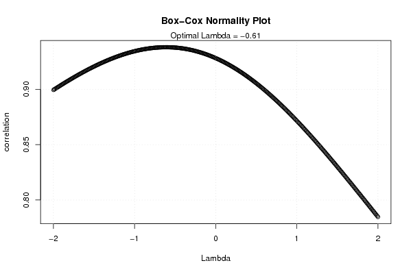
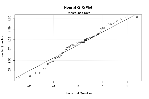
Title produced by software

Box-Cox Normality Plot

Date of computation

Thu, 13 Nov 2008 03:02:49 -0700

Cite this page as follows

Statistical Computations at FreeStatistics.org, Office for Research Development and Education, URL https://freestatistics.org/blog/index.php?v=date/2008/Nov/13/t1226570707hohevncclk673la.htm/, Retrieved Sun, 19 May 2024 12:19:17 +0000

Statistical Computations at FreeStatistics.org, Office for Research Development and Education, URL https://freestatistics.org/blog/index.php?pk=24539, Retrieved Sun, 19 May 2024 12:19:17 +0000

QR Codes:

Paste this QR Code to cite your computation.

Original text written by user:

IsPrivate?

No (this computation is public)

User-defined keywords

Estimated Impact

162

Family? (F = Feedback message, R = changed R code, M = changed R Module, P = changed Parameters, D = changed Data)

F       [Box-Cox Normality Plot] [workshop 3 Q4] [2008-11-13 10:02:49] [1a15026c70cce1c14dcfcc267c5d8133] [Current]

Feedback Forum

2008-11-15 13:34:08 [Ken Wright] [reply] 
Hier laat men lambda ook verschillende waarden aannemen tussen -2 en 2, maar om de gegevens meer normaalverdeeld te maken. De beste waarde voor lambda is -0.61. In dit voorbeeld heeft de transformatie inderdaad wel invloed, je kan goed zien dat het histogram een meer normale verdeling volgt.
2008-11-17 08:26:12 [006ad2c49b6a7c2ad6ab685cfc1dae56] [reply] 
Nu situeert de optimale lambda-waarde voor transformatie zich rond de waarde -0.5 omdat er hier een maximum is. Je kan dus wel stellen dat de verdeling sterk veranderd is.
2008-11-20 09:15:45 [Angelique Van de Vijver] [reply] 
Goede conclusie dat de transformatie heeft gezorgd voor een meer normalere verdeling. Goede interpretatie van de histogrammen en de normal Q-Q-plots. 
Extra uitleg: Op deze box-cox normality plot  is de optimale lambda -0.61. Hier bevindt zich dus het maximum van de kromme, de hoogste correlatie. Als je dan de verschillende histogrammen vergelijkt zie je dat de transformatie wel invloed heeft hier. Het histogram van de originele data heeft een rechtsscheve verdeling, terwijl deze van de getransformeerde data een meer normalere verdeling heeft.  
Je kan dit ook vaststellen op de normal Q-Q plots, waarbij de puntenwolk van de getransformeerde data meer ronde de diagonaal liggen dan de puntenwolk van de originele data.
2008-11-24 12:15:48 [Anouk Greeve] [reply] 
Correcte interpretatie. Wanneer we kunnen spreken van lineariteit in de Normality Plot is er een normale verdeling.

Post a new message

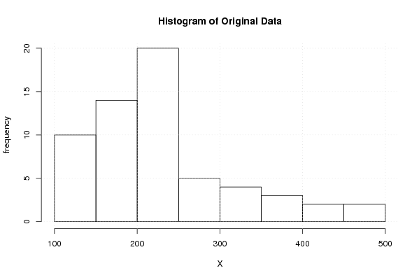
Dataseries X:

Download CSV

Histogram

Boxplots

Summary of computational transaction
Raw Input	view raw input (R code)
Raw Output	view raw output of R engine
Computing time	3 seconds
R Server	'Gwilym Jenkins' @ 72.249.127.135

\begin{tabular}{lllllllll}
\hline
Summary of computational transaction \tabularnewline
Raw Input & view raw input (R code)  \tabularnewline
Raw Output & view raw output of R engine  \tabularnewline
Computing time & 3 seconds \tabularnewline
R Server & 'Gwilym Jenkins' @ 72.249.127.135 \tabularnewline
\hline
\end{tabular}
%Source: https://freestatistics.org/blog/index.php?pk=24539&T=0

[TABLE]
[ROW][C]Summary of computational transaction[/C][/ROW]
[ROW][C]Raw Input[/C][C]view raw input (R code) [/C][/ROW]
[ROW][C]Raw Output[/C][C]view raw output of R engine [/C][/ROW]
[ROW][C]Computing time[/C][C]3 seconds[/C][/ROW]
[ROW][C]R Server[/C][C]'Gwilym Jenkins' @ 72.249.127.135[/C][/ROW]
[/TABLE]
Source: https://freestatistics.org/blog/index.php?pk=24539&T=0

Globally Unique Identifier (entire table): ba.freestatistics.org/blog/index.php?pk=24539&T=0

As an alternative you can also use a QR Code:

The GUIDs for individual cells are displayed in the table below:

Summary of computational transaction
Raw Input	view raw input (R code)
Raw Output	view raw output of R engine
Computing time	3 seconds
R Server	'Gwilym Jenkins' @ 72.249.127.135

Box-Cox Normality Plot
# observations x	60
maximum correlation	0.93798342176156
optimal lambda	-0.61

\begin{tabular}{lllllllll}
\hline
Box-Cox Normality Plot \tabularnewline
# observations x & 60 \tabularnewline
maximum correlation & 0.93798342176156 \tabularnewline
optimal lambda & -0.61 \tabularnewline
\hline
\end{tabular}
%Source: https://freestatistics.org/blog/index.php?pk=24539&T=1

[TABLE]
[ROW][C]Box-Cox Normality Plot[/C][/ROW]
[ROW][C]# observations x[/C][C]60[/C][/ROW]
[ROW][C]maximum correlation[/C][C]0.93798342176156[/C][/ROW]
[ROW][C]optimal lambda[/C][C]-0.61[/C][/ROW]
[/TABLE]
Source: https://freestatistics.org/blog/index.php?pk=24539&T=1

Globally Unique Identifier (entire table): ba.freestatistics.org/blog/index.php?pk=24539&T=1

As an alternative you can also use a QR Code:

The GUIDs for individual cells are displayed in the table below:

Box-Cox Normality Plot
# observations x	60
maximum correlation	0.93798342176156
optimal lambda	-0.61

Figure 1

PNG link

Postscript link

PDF link

Figure 2

PNG link

Postscript link

PDF link

Figure 3

PNG link

Postscript link

PDF link

Figure 4

PNG link

Postscript link

PDF link

Figure 5

PNG link

Postscript link

PDF link

Parameters (Session):

Parameters (R input):

R code (references can be found in the software module):

n <- length(x)
c <- array(NA,dim=c(401))
l <- array(NA,dim=c(401))
mx <- 0
mxli <- -999
for (i in 1:401)
{
l[i] <- (i-201)/100
if (l[i] != 0)
{
x1 <- (x^l[i] - 1) / l[i]
} else {
x1 <- log(x)
}
c[i] <- cor(qnorm(ppoints(x), mean=0, sd=1),x1)
if (mx < c[i])
{
mx <- c[i]
mxli <- l[i]
}
}
c
mx
mxli
if (mxli != 0)
{
x1 <- (x^mxli - 1) / mxli
} else {
x1 <- log(x)
}
bitmap(file='test1.png')
plot(l,c,main='Box-Cox Normality Plot',xlab='Lambda',ylab='correlation')
mtext(paste('Optimal Lambda =',mxli))
grid()
dev.off()
bitmap(file='test2.png')
hist(x,main='Histogram of Original Data',xlab='X',ylab='frequency')
grid()
dev.off()
bitmap(file='test3.png')
hist(x1,main='Histogram of Transformed Data',xlab='X',ylab='frequency')
grid()
dev.off()
bitmap(file='test4.png')
qqnorm(x)
qqline(x)
grid()
mtext('Original Data')
dev.off()
bitmap(file='test5.png')
qqnorm(x1)
qqline(x1)
grid()
mtext('Transformed Data')
dev.off()
load(file='createtable')
a<-table.start()
a<-table.row.start(a)
a<-table.element(a,'Box-Cox Normality Plot',2,TRUE)
a<-table.row.end(a)
a<-table.row.start(a)
a<-table.element(a,'# observations x',header=TRUE)
a<-table.element(a,n)
a<-table.row.end(a)
a<-table.row.start(a)
a<-table.element(a,'maximum correlation',header=TRUE)
a<-table.element(a,mx)
a<-table.row.end(a)
a<-table.row.start(a)
a<-table.element(a,'optimal lambda',header=TRUE)
a<-table.element(a,mxli)
a<-table.row.end(a)
a<-table.end(a)
table.save(a,file='mytable.tab')

Free Statistics

Description of Statistical Computation

Tree of Dependent Computations

Dataset

Tables (Output of Computation)

Figures (Output of Computation)

Input Parameters & R Code