Free Statistics
of Irreproducible Research!
Description of Statistical Computation | |||||||||||||||||||||||||||||||||||||||||||||
|---|---|---|---|---|---|---|---|---|---|---|---|---|---|---|---|---|---|---|---|---|---|---|---|---|---|---|---|---|---|---|---|---|---|---|---|---|---|---|---|---|---|---|---|---|---|
| Author's title | |||||||||||||||||||||||||||||||||||||||||||||
| Author | *The author of this computation has been verified* | ||||||||||||||||||||||||||||||||||||||||||||
| R Software Module | rwasp_boxcoxlin.wasp | ||||||||||||||||||||||||||||||||||||||||||||
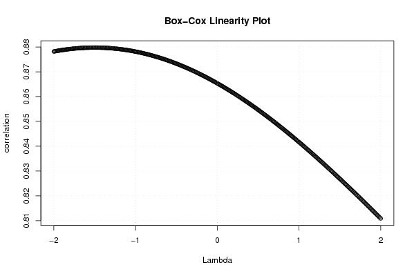
| Title produced by software | Box-Cox Linearity Plot | ||||||||||||||||||||||||||||||||||||||||||||
| Date of computation | Thu, 13 Nov 2008 02:25:57 -0700 | ||||||||||||||||||||||||||||||||||||||||||||
| Cite this page as follows | Statistical Computations at FreeStatistics.org, Office for Research Development and Education, URL https://freestatistics.org/blog/index.php?v=date/2008/Nov/13/t1226568430wve6bpb9zjjbiec.htm/, Retrieved Fri, 04 Jul 2025 02:35:38 +0000 | ||||||||||||||||||||||||||||||||||||||||||||
| Statistical Computations at FreeStatistics.org, Office for Research Development and Education, URL https://freestatistics.org/blog/index.php?pk=24514, Retrieved Fri, 04 Jul 2025 02:35:38 +0000 | |||||||||||||||||||||||||||||||||||||||||||||
| QR Codes: | |||||||||||||||||||||||||||||||||||||||||||||
|
| |||||||||||||||||||||||||||||||||||||||||||||
| Original text written by user: | |||||||||||||||||||||||||||||||||||||||||||||
| IsPrivate? | No (this computation is public) | ||||||||||||||||||||||||||||||||||||||||||||
| User-defined keywords | |||||||||||||||||||||||||||||||||||||||||||||
| Estimated Impact | 291 | ||||||||||||||||||||||||||||||||||||||||||||
Tree of Dependent Computations | |||||||||||||||||||||||||||||||||||||||||||||
| Family? (F = Feedback message, R = changed R code, M = changed R Module, P = changed Parameters, D = changed Data) | |||||||||||||||||||||||||||||||||||||||||||||
| F [Box-Cox Linearity Plot] [W3Q3] [2008-11-13 09:25:57] [434228f9e3c7eaa307f0fb12855e2147] [Current] - RMPD [Testing Mean with known Variance - Critical Value] [W4Q1] [2008-11-13 09:49:36] [88cf507fbedaeeb6f794e4dc3641d02c] - RMPD [Testing Mean with known Variance - p-value] [W4Q2] [2008-11-13 09:56:06] [fefc9cefce013a6daab207c2a2eec05e] - RMPD [Testing Mean with known Variance - Type II Error] [W4Q3] [2008-11-13 10:00:09] [fefc9cefce013a6daab207c2a2eec05e] | |||||||||||||||||||||||||||||||||||||||||||||
| Feedback Forum | |||||||||||||||||||||||||||||||||||||||||||||
Post a new message | |||||||||||||||||||||||||||||||||||||||||||||
Dataset | |||||||||||||||||||||||||||||||||||||||||||||
| Dataseries X: | |||||||||||||||||||||||||||||||||||||||||||||
118,4 121,4 128,8 131,7 141,7 142,9 139,4 134,7 125,0 113,6 111,5 108,5 112,3 116,6 115,5 120,1 132,9 128,1 129,3 132,5 131,0 124,9 120,8 122,0 122,1 127,4 135,2 137,3 135,0 136,0 138,4 134,7 138,4 133,9 133,6 141,2 151,8 155,4 156,6 161,6 160,7 156,0 159,5 168,7 169,9 169,9 185,9 190,8 195,8 211,9 227,1 251,3 256,7 251,9 251,2 270,3 267,2 243,0 229,9 187,2 | |||||||||||||||||||||||||||||||||||||||||||||
| Dataseries Y: | |||||||||||||||||||||||||||||||||||||||||||||
111,4 114,1 121,8 127,6 129,9 128,0 123,5 124,0 127,4 127,6 128,4 131,4 135,1 134,0 144,5 147,3 150,9 148,7 141,4 138,9 139,8 145,6 147,9 148,5 151,1 157,5 167,5 172,3 173,5 187,5 205,5 195,1 204,5 204,5 201,7 207,0 206,6 210,6 211,1 215,0 223,9 238,2 238,9 229,6 232,2 222,1 221,6 227,3 221,0 213,6 243,4 253,8 265,3 268,2 268,5 266,9 268,4 250,8 231,2 192,0 | |||||||||||||||||||||||||||||||||||||||||||||
Tables (Output of Computation) | |||||||||||||||||||||||||||||||||||||||||||||
| |||||||||||||||||||||||||||||||||||||||||||||
Figures (Output of Computation) | |||||||||||||||||||||||||||||||||||||||||||||
Input Parameters & R Code | |||||||||||||||||||||||||||||||||||||||||||||
| Parameters (Session): | |||||||||||||||||||||||||||||||||||||||||||||
| Parameters (R input): | |||||||||||||||||||||||||||||||||||||||||||||
| R code (references can be found in the software module): | |||||||||||||||||||||||||||||||||||||||||||||
n <- length(x) | |||||||||||||||||||||||||||||||||||||||||||||