Repository of Reproducible Computations

Free Statistics

of Irreproducible Research!

Author's title

Author

*The author of this computation has been verified*

R Software Module

rwasp_boxcoxlin.wasp

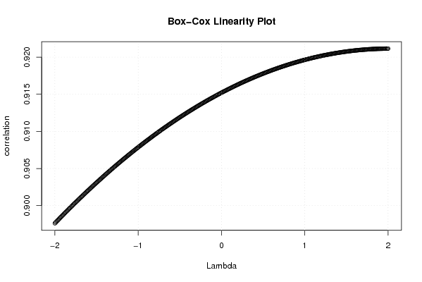
Title produced by software

Box-Cox Linearity Plot

Date of computation

Wed, 12 Nov 2008 11:42:43 -0700

Cite this page as follows

Statistical Computations at FreeStatistics.org, Office for Research Development and Education, URL https://freestatistics.org/blog/index.php?v=date/2008/Nov/12/t1226515415xl6nkzn2j230ozo.htm/, Retrieved Sun, 19 May 2024 09:17:12 +0000

Statistical Computations at FreeStatistics.org, Office for Research Development and Education, URL https://freestatistics.org/blog/index.php?pk=24373, Retrieved Sun, 19 May 2024 09:17:12 +0000

QR Codes:

Paste this QR Code to cite your computation.

Original text written by user:

IsPrivate?

No (this computation is public)

User-defined keywords

Box cox

Estimated Impact

137

Family? (F = Feedback message, R = changed R code, M = changed R Module, P = changed Parameters, D = changed Data)

F       [Box-Cox Linearity Plot] [workshop 2 Q3 Box...] [2008-11-12 18:42:43] [74c7506a1ea162af3aa8be25bcd05d28] [Current]

Feedback Forum

2008-11-15 11:58:37 [58d427c57bd46519a715a3a7fea6a80f] [reply] 
transformeren. De nieuwe lijn is misschien wel een kromme. De box-cox transformatie kan wel wat problemen oplossen R-code x wordt getransformeerd. Correlatie kan je aflezen op de y-as. We hopen op een maximum, in dit geval is die waarschijnlijk 2. Deze transformatie brengt niet veel verbetering.
2008-11-19 18:54:53 [Bénédicte Soens] [reply] 
2 variabelen worden in verband gebracht met elkaar in een scatterplot en door de punten wordt een lijn getrokken (=wetmatigheid vertonen). Uit de originele data kan men zien dat er heel wat punten niet op de lijn liggen, vandaar dan ook de kromme bij de box-cox linearity plot. Deze lijkt sterkt op de helft van een parabool. Op de y-as is de correlatie te vinden en op e x-as de lambda, die tussen -2 en 2 gelegen is (daartussen berekenen). Aangezien er hier een parabool is weergegeven waarvan de top duidelijk zichtbaar is, kan men zeggen dat er een zinvolle transformatie zal hebben plaats gevonden. Welke transformatie er is toegepast kan men zien in de R-code, hier was het een logaritme. Hier zal de transformatie de correlatie niet veel verhoogd hebben, dit is ook te zien aan de grafiek met de originele data t.o.v deze van de getransformeerde data (punten nog steeds vrij ver verspreid).
2008-11-24 11:58:22 [Julian De Ruyter] [reply] 
Beknopte conclusie bij de figuur gegeven door de student.  
De box-cox lineairity plot probeert een variabele X te transformeren zodat het effect van correlatie hierdoor tussen 2variabelen hopelijk verhoogt wordt.  
X-as = lamdba en Y-as is de correlatie tussen getransformeerde x en originele y. We gaan lambda tussen 2 en -2 laten verschuiven om een maximum in de functie te bekomen. 
De gegevens blijven min of meer hetzelfde. De transformatie heeft met andere woorden niet veel uitgehaald...  
 

Post a new message

Dataseries X:

Download CSV

Histogram

Boxplots

8,4
8,4
8,4
8,6
8,9
8,8
8,3
7,5
7,2
7,5
8,8
9,3
9,3
8,7
8,2
8,3
8,5
8,6
8,6
8,2
8,1
8
8,6
8,7
8,8
8,5
8,4
8,5
8,7
8,7
8,6
8,5
8,3
8,1
8,2
8,1
8,1
7,9
7,9
7,9
8
8
7,9
8
7,7
7,2
7,5
7,3
7
7
7
7,2
7,3
7,1
6,8
6,6
6,2
6,2
6,8
6,9
6,8

Dataseries Y:

Download CSV

Histogram

7,6
7,9
7,9
8,1
8,2
8
7,5
6,8
6,5
6,6
7,6
8
8
7,7
7,5
7,6
7,7
7,9
7,8
7,5
7,5
7,1
7,5
7,5
7,6
7,7
7,7
7,9
8,1
8,2
8,2
8,1
7,9
7,3
6,9
6,6
6,7
6,9
7
7,1
7,2
7,1
6,9
7
6,8
6,4
6,7
6,7
6,4
6,3
6,2
6,5
6,8
6,8
6,5
6,3
5,9
5,9
6,4
6,4
6,5

Summary of computational transaction
Raw Input	view raw input (R code)
Raw Output	view raw output of R engine
Computing time	1 seconds
R Server	'Gwilym Jenkins' @ 72.249.127.135

\begin{tabular}{lllllllll}
\hline
Summary of computational transaction \tabularnewline
Raw Input & view raw input (R code)  \tabularnewline
Raw Output & view raw output of R engine  \tabularnewline
Computing time & 1 seconds \tabularnewline
R Server & 'Gwilym Jenkins' @ 72.249.127.135 \tabularnewline
\hline
\end{tabular}
%Source: https://freestatistics.org/blog/index.php?pk=24373&T=0

[TABLE]
[ROW][C]Summary of computational transaction[/C][/ROW]
[ROW][C]Raw Input[/C][C]view raw input (R code) [/C][/ROW]
[ROW][C]Raw Output[/C][C]view raw output of R engine [/C][/ROW]
[ROW][C]Computing time[/C][C]1 seconds[/C][/ROW]
[ROW][C]R Server[/C][C]'Gwilym Jenkins' @ 72.249.127.135[/C][/ROW]
[/TABLE]
Source: https://freestatistics.org/blog/index.php?pk=24373&T=0

Globally Unique Identifier (entire table): ba.freestatistics.org/blog/index.php?pk=24373&T=0

As an alternative you can also use a QR Code:

The GUIDs for individual cells are displayed in the table below:

Summary of computational transaction
Raw Input	view raw input (R code)
Raw Output	view raw output of R engine
Computing time	1 seconds
R Server	'Gwilym Jenkins' @ 72.249.127.135

Box-Cox Linearity Plot
# observations x	61
maximum correlation	0.92115182894294
optimal lambda(x)	2
Residual SD (orginial)	0.255333537654387
Residual SD (transformed)	0.253019035153299

\begin{tabular}{lllllllll}
\hline
Box-Cox Linearity Plot \tabularnewline
# observations x & 61 \tabularnewline
maximum correlation & 0.92115182894294 \tabularnewline
optimal lambda(x) & 2 \tabularnewline
Residual SD (orginial) & 0.255333537654387 \tabularnewline
Residual SD (transformed) & 0.253019035153299 \tabularnewline
\hline
\end{tabular}
%Source: https://freestatistics.org/blog/index.php?pk=24373&T=1

[TABLE]
[ROW][C]Box-Cox Linearity Plot[/C][/ROW]
[ROW][C]# observations x[/C][C]61[/C][/ROW]
[ROW][C]maximum correlation[/C][C]0.92115182894294[/C][/ROW]
[ROW][C]optimal lambda(x)[/C][C]2[/C][/ROW]
[ROW][C]Residual SD (orginial)[/C][C]0.255333537654387[/C][/ROW]
[ROW][C]Residual SD (transformed)[/C][C]0.253019035153299[/C][/ROW]
[/TABLE]
Source: https://freestatistics.org/blog/index.php?pk=24373&T=1

Globally Unique Identifier (entire table): ba.freestatistics.org/blog/index.php?pk=24373&T=1

As an alternative you can also use a QR Code:

The GUIDs for individual cells are displayed in the table below:

Box-Cox Linearity Plot
# observations x	61
maximum correlation	0.92115182894294
optimal lambda(x)	2
Residual SD (orginial)	0.255333537654387
Residual SD (transformed)	0.253019035153299

Figure 1

PNG link

Postscript link

PDF link

Figure 2

PNG link

Postscript link

PDF link

Figure 3

PNG link

Postscript link

PDF link

Parameters (Session):

Parameters (R input):

R code (references can be found in the software module):

n <- length(x)
c <- array(NA,dim=c(401))
l <- array(NA,dim=c(401))
mx <- 0
mxli <- -999
for (i in 1:401)
{
l[i] <- (i-201)/100
if (l[i] != 0)
{
x1 <- (x^l[i] - 1) / l[i]
} else {
x1 <- log(x)
}
c[i] <- cor(x1,y)
if (mx < abs(c[i]))
{
mx <- abs(c[i])
mxli <- l[i]
}
}
c
mx
mxli
if (mxli != 0)
{
x1 <- (x^mxli - 1) / mxli
} else {
x1 <- log(x)
}
r<-lm(y~x)
se <- sqrt(var(r$residuals))
r1 <- lm(y~x1)
se1 <- sqrt(var(r1$residuals))
bitmap(file='test1.png')
plot(l,c,main='Box-Cox Linearity Plot',xlab='Lambda',ylab='correlation')
grid()
dev.off()
bitmap(file='test2.png')
plot(x,y,main='Linear Fit of Original Data',xlab='x',ylab='y')
abline(r)
grid()
mtext(paste('Residual Standard Deviation = ',se))
dev.off()
bitmap(file='test3.png')
plot(x1,y,main='Linear Fit of Transformed Data',xlab='x',ylab='y')
abline(r1)
grid()
mtext(paste('Residual Standard Deviation = ',se1))
dev.off()
load(file='createtable')
a<-table.start()
a<-table.row.start(a)
a<-table.element(a,'Box-Cox Linearity Plot',2,TRUE)
a<-table.row.end(a)
a<-table.row.start(a)
a<-table.element(a,'# observations x',header=TRUE)
a<-table.element(a,n)
a<-table.row.end(a)
a<-table.row.start(a)
a<-table.element(a,'maximum correlation',header=TRUE)
a<-table.element(a,mx)
a<-table.row.end(a)
a<-table.row.start(a)
a<-table.element(a,'optimal lambda(x)',header=TRUE)
a<-table.element(a,mxli)
a<-table.row.end(a)
a<-table.row.start(a)
a<-table.element(a,'Residual SD (orginial)',header=TRUE)
a<-table.element(a,se)
a<-table.row.end(a)
a<-table.row.start(a)
a<-table.element(a,'Residual SD (transformed)',header=TRUE)
a<-table.element(a,se1)
a<-table.row.end(a)
a<-table.end(a)
table.save(a,file='mytable.tab')

Free Statistics

Description of Statistical Computation

Tree of Dependent Computations

Dataset

Tables (Output of Computation)

Figures (Output of Computation)

Input Parameters & R Code