• QR Code (size=2)
• QR Code (size=3)
• QR Code (size=4)
• QR Code (size=5)
• QR Code (size=6)

90,7
94,3
104,6
111,1
110,8
107,2
99
99
91
96,2
96,9
96,2
100,1
99
115,4
106,9
107,1
99,3
99,2
108,3
105,6
99,5
107,4
93,1
88,1
110,7
113,1
99,6
93,6
98,6
99,6
114,3
107,8
101,2
112,5
100,5
93,9
116,2
112
106,4
95,7
96
95,8
103
102,2
98,4
111,4
86,6
91,3
107,9
101,8
104,4
93,4
100,1
98,5
112,9
101,4
107,1
110,8
90,3
95,5
111,4
113
107,5
95,9
106,3
105,2
117,2
106,9
108,2
113
97,2
99,9
108,1
118,1
109,1
93,3
112,1
111,8
112,5
116,3
110,3
117,1
103,4
96,2

78,4
114,6
113,3
117
99,6
99,4
101,9
115,2
108,5
113,8
121
92,2
90,2
101,5
126,6
93,9
89,8
93,4
101,5
110,4
105,9
108,4
113,9
86,1
69,4
101,2
100,5
98
106,6
90,1
96,9
125,9
112
100
123,9
79,8
83,4
113,6
112,9
104
109,9
99
106,3
128,9
111,1
102,9
130
87
87,5
117,6
103,4
110,8
112,6
102,5
112,4
135,6
105,1
127,7
137
91
90,5
122,4
123,3
124,3
120
118,1
119
142,7
123,6
129,6
151,6
110,4
99,2
130,5
136,2
129,7
128
121,6
135,8
143,8
147,5
136,2
156,6
123,3
100,4

97,8
107,4
117,5
105,6
97,4
99,5
98
104,3
100,6
101,1
103,9
96,9
95,5
108,4
117
103,8
100,8
110,6
104
112,6
107,3
98,9
109,8
104,9
102,2
123,9
124,9
112,7
121,9
100,6
104,3
120,4
107,5
102,9
125,6
107,5
108,8
128,4
121,1
119,5
128,7
108,7
105,5
119,8
111,3
110,6
120,1
97,5
107,7
127,3
117,2
119,8
116,2
111
112,4
130,6
109,1
118,8
123,9
101,6
112,8
128
129,6
125,8
119,5
115,7
113,6
129,7
112
116,8
127
112,1
114,2
121,1
131,6
125
120,4
117,7
117,5
120,6
127,5
112,3
124,5
115,2
105,4

x <- array(x,dim=c(length(x),1))
colnames(x) <- par5
y <- array(y,dim=c(length(y),1))
colnames(y) <- par6
z <- array(z,dim=c(length(z),1))
colnames(z) <- par7
d <- data.frame(cbind(z,y,x))
colnames(d) <- list(par7,par6,par5)
par1 <- as.numeric(par1)
par2 <- as.numeric(par2)
if (par1>500) par1 <- 500
if (par2>500) par2 <- 500
if (par1<10) par1 <- 10
if (par2<10) par2 <- 10
library(GenKern)
library(lattice)
panel.hist <- function(x, ...)
{
usr <- par('usr'); on.exit(par(usr))
par(usr = c(usr[1:2], 0, 1.5) )
h <- hist(x, plot = FALSE)
breaks <- h$breaks; nB <- length(breaks)
y <- h$counts; y <- y/max(y)
rect(breaks[-nB], 0, breaks[-1], y, col='black', ...)
}
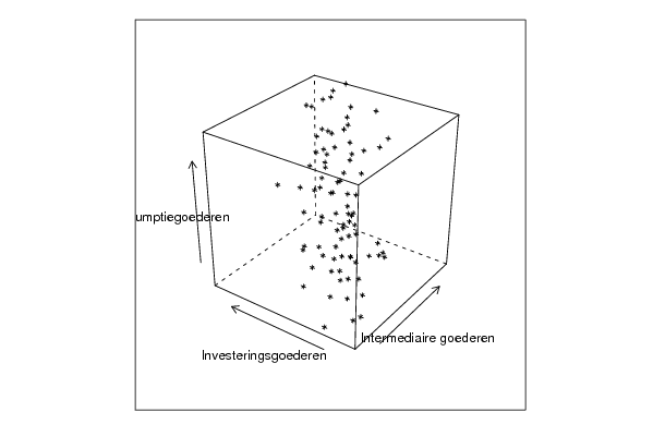
bitmap(file='cloud1.png')
cloud(z~x*y, screen = list(x=-45, y=45, z=35),xlab=par5,ylab=par6,zlab=par7)
dev.off()
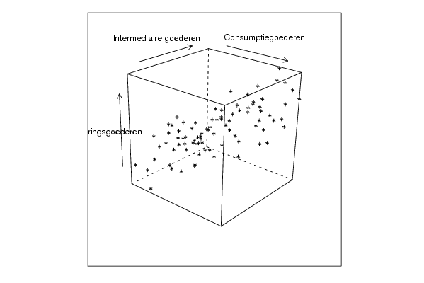
bitmap(file='cloud2.png')
cloud(z~x*y, screen = list(x=35, y=45, z=25),xlab=par5,ylab=par6,zlab=par7)
dev.off()
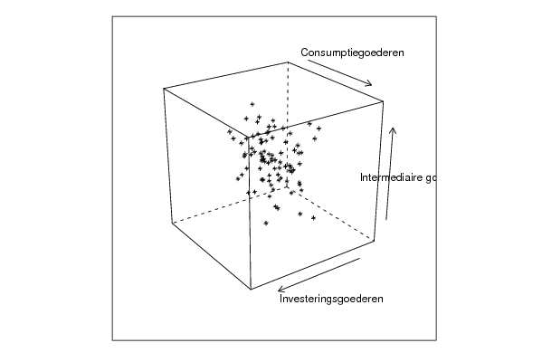
bitmap(file='cloud3.png')
cloud(z~x*y, screen = list(x=35, y=-25, z=90),xlab=par5,ylab=par6,zlab=par7)
dev.off()
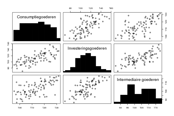
bitmap(file='pairs.png')
pairs(d,diag.panel=panel.hist)
dev.off()
x <- as.vector(x)
y <- as.vector(y)
z <- as.vector(z)
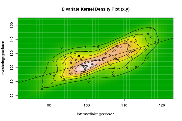
bitmap(file='bidensity1.png')
op <- KernSur(x,y, xgridsize=par1, ygridsize=par2, correlation=cor(x,y), xbandwidth=dpik(x), ybandwidth=dpik(y))
image(op$xords, op$yords, op$zden, col=terrain.colors(100), axes=TRUE,main='Bivariate Kernel Density Plot (x,y)',xlab=par5,ylab=par6)
if (par3=='Y') contour(op$xords, op$yords, op$zden, add=TRUE)
if (par4=='Y') points(x,y)
(r<-lm(y ~ x))
abline(r)
box()
dev.off()
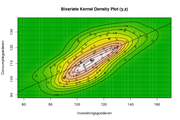
bitmap(file='bidensity2.png')
op <- KernSur(y,z, xgridsize=par1, ygridsize=par2, correlation=cor(y,z), xbandwidth=dpik(y), ybandwidth=dpik(z))
op
image(op$xords, op$yords, op$zden, col=terrain.colors(100), axes=TRUE,main='Bivariate Kernel Density Plot (y,z)',xlab=par6,ylab=par7)
if (par3=='Y') contour(op$xords, op$yords, op$zden, add=TRUE)
if (par4=='Y') points(y,z)
(r<-lm(z ~ y))
abline(r)
box()
dev.off()
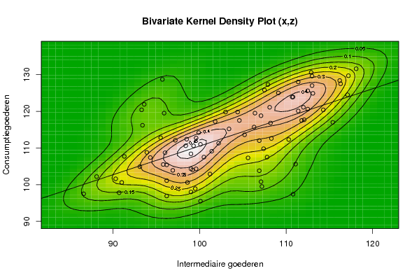
bitmap(file='bidensity3.png')
op <- KernSur(x,z, xgridsize=par1, ygridsize=par2, correlation=cor(x,z), xbandwidth=dpik(x), ybandwidth=dpik(z))
op
image(op$xords, op$yords, op$zden, col=terrain.colors(100), axes=TRUE,main='Bivariate Kernel Density Plot (x,z)',xlab=par5,ylab=par7)
if (par3=='Y') contour(op$xords, op$yords, op$zden, add=TRUE)
if (par4=='Y') points(x,z)
(r<-lm(z ~ x))
abline(r)
box()
dev.off()