Free Statistics
of Irreproducible Research!
Description of Statistical Computation | |||||||||||||||||||||||||||||||||||||
|---|---|---|---|---|---|---|---|---|---|---|---|---|---|---|---|---|---|---|---|---|---|---|---|---|---|---|---|---|---|---|---|---|---|---|---|---|---|
| Author's title | |||||||||||||||||||||||||||||||||||||
| Author | *Unverified author* | ||||||||||||||||||||||||||||||||||||
| R Software Module | rwasp_boxcoxnorm.wasp | ||||||||||||||||||||||||||||||||||||
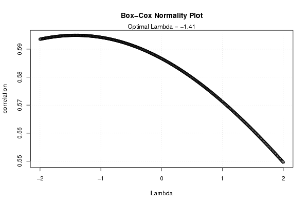
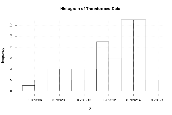
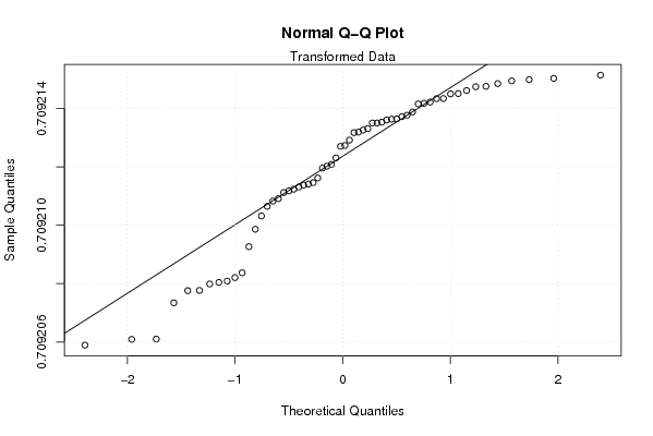
| Title produced by software | Box-Cox Normality Plot | ||||||||||||||||||||||||||||||||||||
| Date of computation | Wed, 12 Nov 2008 10:53:57 -0700 | ||||||||||||||||||||||||||||||||||||
| Cite this page as follows | Statistical Computations at FreeStatistics.org, Office for Research Development and Education, URL https://freestatistics.org/blog/index.php?v=date/2008/Nov/12/t1226512468q3pzsercyugitxq.htm/, Retrieved Sun, 19 May 2024 08:50:22 +0000 | ||||||||||||||||||||||||||||||||||||
| Statistical Computations at FreeStatistics.org, Office for Research Development and Education, URL https://freestatistics.org/blog/index.php?pk=24328, Retrieved Sun, 19 May 2024 08:50:22 +0000 | |||||||||||||||||||||||||||||||||||||
| QR Codes: | |||||||||||||||||||||||||||||||||||||
|
| |||||||||||||||||||||||||||||||||||||
| Original text written by user: | |||||||||||||||||||||||||||||||||||||
| IsPrivate? | No (this computation is public) | ||||||||||||||||||||||||||||||||||||
| User-defined keywords | |||||||||||||||||||||||||||||||||||||
| Estimated Impact | 163 | ||||||||||||||||||||||||||||||||||||
Tree of Dependent Computations | |||||||||||||||||||||||||||||||||||||
| Family? (F = Feedback message, R = changed R code, M = changed R Module, P = changed Parameters, D = changed Data) | |||||||||||||||||||||||||||||||||||||
| - [Bivariate Kernel Density Estimation] [Bel20 en Downjones] [2008-11-12 17:23:23] [74be16979710d4c4e7c6647856088456] F RMPD [Box-Cox Normality Plot] [kelly] [2008-11-12 17:53:57] [d41d8cd98f00b204e9800998ecf8427e] [Current] F D [Box-Cox Normality Plot] [Box cox normality...] [2008-11-13 22:31:24] [74be16979710d4c4e7c6647856088456] | |||||||||||||||||||||||||||||||||||||
| Feedback Forum | |||||||||||||||||||||||||||||||||||||
Post a new message | |||||||||||||||||||||||||||||||||||||
Dataset | |||||||||||||||||||||||||||||||||||||
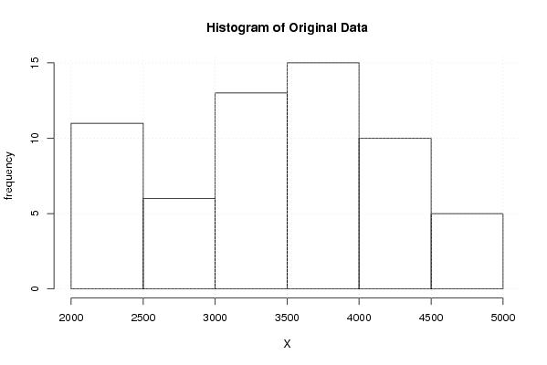
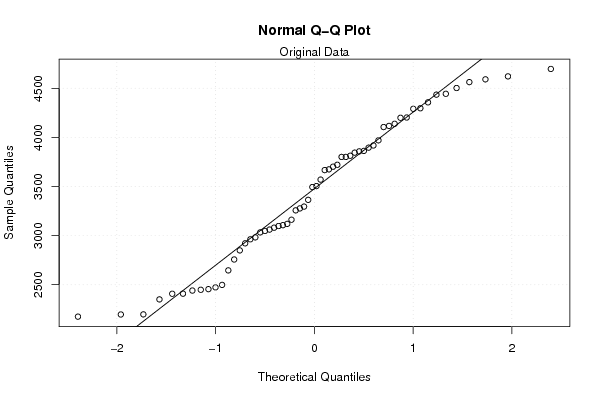
| Dataseries X: | |||||||||||||||||||||||||||||||||||||
2174,56 2196,72 2350,44 2440,25 2408,64 2472,81 2407,6 2454,62 2448,05 2497,84 2645,64 2756,76 2849,27 2921,44 2981,85 3080,58 3106,22 3119,31 3061,26 3097,31 3161,69 3257,16 3277,01 3295,32 3363,99 3494,17 3667,03 3813,06 3917,96 3895,51 3801,06 3570,12 3701,61 3862,27 3970,1 4138,52 4199,75 4290,89 4443,91 4502,64 4356,98 4591,27 4696,96 4621,4 4562,84 4202,52 4296,49 4435,23 4105,18 4116,68 3844,49 3720,98 3674,4 3857,62 3801,06 3504,37 3032,6 3047,03 2962,34 2197,82 | |||||||||||||||||||||||||||||||||||||
Tables (Output of Computation) | |||||||||||||||||||||||||||||||||||||
| |||||||||||||||||||||||||||||||||||||
Figures (Output of Computation) | |||||||||||||||||||||||||||||||||||||
Input Parameters & R Code | |||||||||||||||||||||||||||||||||||||
| Parameters (Session): | |||||||||||||||||||||||||||||||||||||
| Parameters (R input): | |||||||||||||||||||||||||||||||||||||
| R code (references can be found in the software module): | |||||||||||||||||||||||||||||||||||||
n <- length(x) | |||||||||||||||||||||||||||||||||||||