Free Statistics
of Irreproducible Research!
Description of Statistical Computation | |||||||||||||||||||||
|---|---|---|---|---|---|---|---|---|---|---|---|---|---|---|---|---|---|---|---|---|---|
| Author's title | |||||||||||||||||||||
| Author | *The author of this computation has been verified* | ||||||||||||||||||||
| R Software Module | rwasp_cloud.wasp | ||||||||||||||||||||
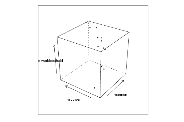
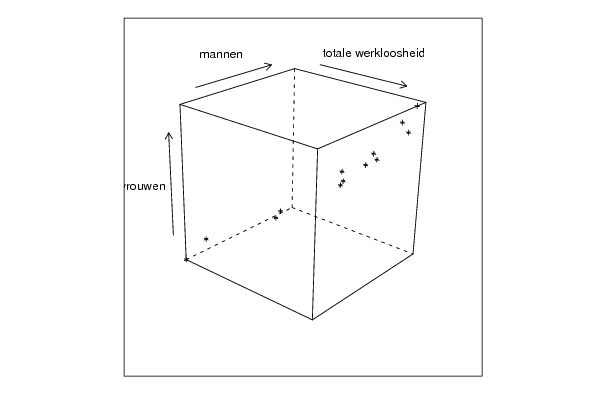
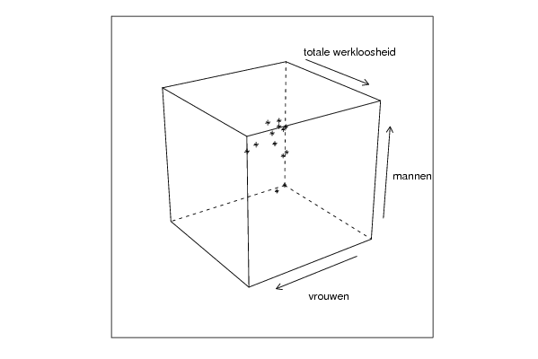
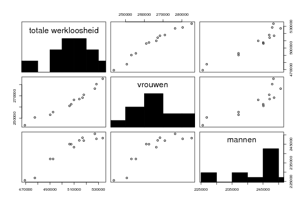
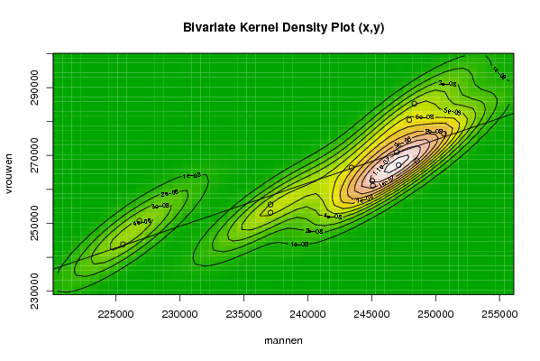
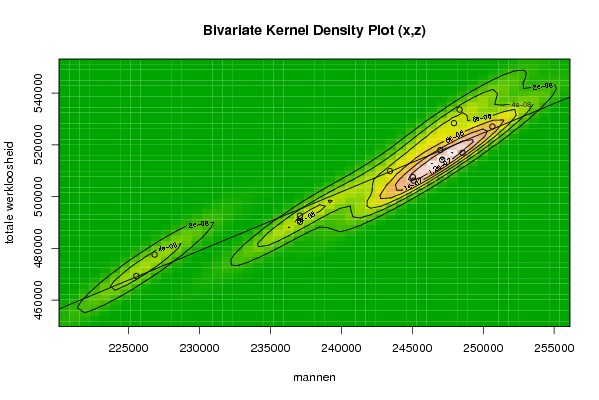
| Title produced by software | Trivariate Scatterplots | ||||||||||||||||||||
| Date of computation | Wed, 12 Nov 2008 02:06:38 -0700 | ||||||||||||||||||||
| Cite this page as follows | Statistical Computations at FreeStatistics.org, Office for Research Development and Education, URL https://freestatistics.org/blog/index.php?v=date/2008/Nov/12/t12264808489f8z2t5q51mwye7.htm/, Retrieved Sun, 19 May 2024 11:32:23 +0000 | ||||||||||||||||||||
| Statistical Computations at FreeStatistics.org, Office for Research Development and Education, URL https://freestatistics.org/blog/index.php?pk=24022, Retrieved Sun, 19 May 2024 11:32:23 +0000 | |||||||||||||||||||||
| QR Codes: | |||||||||||||||||||||
|
| |||||||||||||||||||||
| Original text written by user: | |||||||||||||||||||||
| IsPrivate? | No (this computation is public) | ||||||||||||||||||||
| User-defined keywords | werkloosheid mannen en vrouwen julie govaerts | ||||||||||||||||||||
| Estimated Impact | 214 | ||||||||||||||||||||
Tree of Dependent Computations | |||||||||||||||||||||
| Family? (F = Feedback message, R = changed R code, M = changed R Module, P = changed Parameters, D = changed Data) | |||||||||||||||||||||
| - [Trivariate Scatterplots] [trivariate scatte...] [2008-11-12 09:06:38] [ff1af8c6f1c2f1c0e8def9bfc9355be9] [Current] F RMPD [Partial Correlation] [Q1 various ECA to...] [2008-11-12 14:29:07] [b478325fa744e3f2fc16a7222294469c] | |||||||||||||||||||||
| Feedback Forum | |||||||||||||||||||||
Post a new message | |||||||||||||||||||||
Dataset | |||||||||||||||||||||
| Dataseries X: | |||||||||||||||||||||
250643 243422 247105 248541 245039 237080 237085 225554 226839 247934 248333 246969 245098 | |||||||||||||||||||||
| Dataseries Y: | |||||||||||||||||||||
276427 266424 267153 268381 262522 255542 253158 243803 250741 280445 285257 270976 261076 | |||||||||||||||||||||
| Dataseries Z: | |||||||||||||||||||||
527070 509846 514258 516922 507561 492622 490243 469357 477580 528379 533590 517945 506174 | |||||||||||||||||||||
Tables (Output of Computation) | |||||||||||||||||||||
| |||||||||||||||||||||
Figures (Output of Computation) | |||||||||||||||||||||
Input Parameters & R Code | |||||||||||||||||||||
| Parameters (Session): | |||||||||||||||||||||
| par1 = 50 ; par2 = 50 ; par3 = Y ; par4 = Y ; par5 = mannen ; par6 = vrouwen ; par7 = totale werkloosheid ; | |||||||||||||||||||||
| Parameters (R input): | |||||||||||||||||||||
| par1 = 50 ; par2 = 50 ; par3 = Y ; par4 = Y ; par5 = mannen ; par6 = vrouwen ; par7 = totale werkloosheid ; | |||||||||||||||||||||
| R code (references can be found in the software module): | |||||||||||||||||||||
x <- array(x,dim=c(length(x),1)) | |||||||||||||||||||||