Free Statistics
of Irreproducible Research!
Description of Statistical Computation | |||||||||||||||||||||
|---|---|---|---|---|---|---|---|---|---|---|---|---|---|---|---|---|---|---|---|---|---|
| Author's title | |||||||||||||||||||||
| Author | *The author of this computation has been verified* | ||||||||||||||||||||
| R Software Module | rwasp_cloud.wasp | ||||||||||||||||||||
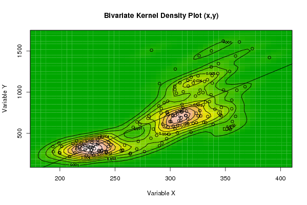
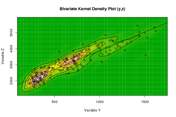
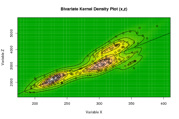
| Title produced by software | Trivariate Scatterplots | ||||||||||||||||||||
| Date of computation | Tue, 11 Nov 2008 14:02:37 -0700 | ||||||||||||||||||||
| Cite this page as follows | Statistical Computations at FreeStatistics.org, Office for Research Development and Education, URL https://freestatistics.org/blog/index.php?v=date/2008/Nov/11/t1226437937rn4trfsgfe47oxi.htm/, Retrieved Sun, 19 May 2024 12:34:35 +0000 | ||||||||||||||||||||
| Statistical Computations at FreeStatistics.org, Office for Research Development and Education, URL https://freestatistics.org/blog/index.php?pk=23980, Retrieved Sun, 19 May 2024 12:34:35 +0000 | |||||||||||||||||||||
| QR Codes: | |||||||||||||||||||||
|
| |||||||||||||||||||||
| Original text written by user: | |||||||||||||||||||||
| IsPrivate? | No (this computation is public) | ||||||||||||||||||||
| User-defined keywords | |||||||||||||||||||||
| Estimated Impact | 163 | ||||||||||||||||||||
Tree of Dependent Computations | |||||||||||||||||||||
| Family? (F = Feedback message, R = changed R code, M = changed R Module, P = changed Parameters, D = changed Data) | |||||||||||||||||||||
| F [Mean Plot] [workshop 3] [2007-10-26 12:14:28] [e9ffc5de6f8a7be62f22b142b5b6b1a8] F R PD [Mean Plot] [vraag 2] [2008-10-29 19:00:24] [c45c87b96bbf32ffc2144fc37d767b2e] F R P [Mean Plot] [vraag 4] [2008-10-29 22:25:49] [c45c87b96bbf32ffc2144fc37d767b2e] F R PD [Mean Plot] [taak 5] [2008-10-30 06:53:19] [c45c87b96bbf32ffc2144fc37d767b2e] - RMPD [Trivariate Scatterplots] [] [2008-11-11 21:02:37] [c60a842d48931bd392d024d8e9ef4583] [Current] | |||||||||||||||||||||
| Feedback Forum | |||||||||||||||||||||
Post a new message | |||||||||||||||||||||
Dataset | |||||||||||||||||||||
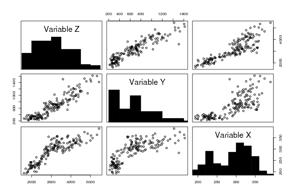
| Dataseries X: | |||||||||||||||||||||
227.3 222.9 263.6 208.6 242 245.6 199.5 213.6 241.9 242 230.6 193.9 235.5 228.3 227.3 215.7 219.3 218 215.4 193.6 225.7 235.8 211.9 199.1 222.5 217.9 229 244.3 220.8 234.3 215.2 201.7 258.6 271 228.7 230.3 243.9 231.3 276.6 256.9 238 256.7 233.8 199.9 263.9 255.6 237.7 229.2 223.9 235.2 290.2 269.6 246.3 287.7 234.3 238.3 296.7 282.5 292.5 298.9 284.7 309.5 356.3 302.6 345.3 353.9 297.2 299.6 355.8 348.3 340.5 310.1 323.5 307.9 354.5 298 306.6 302.3 291.7 280.7 311.5 334 320.8 266.4 318.9 306.4 338.9 330.3 314.4 316 310 272.4 327.6 343.9 315.8 279.8 323.7 300.6 326.8 314.7 293.1 313.9 304.7 269.9 332.2 346.5 295.8 297.9 304.3 306.7 359.2 325.3 302.4 351.2 310.8 289.6 355.8 335.5 332 310.7 297.1 291.9 326 311.8 294.5 330 297.7 290.3 338 319 316.3 304.3 305.6 304 353.8 308.7 325.2 337.2 304.6 320.8 327.1 360.4 346.3 325.2 322.9 337 367.8 329.7 333.7 338.1 331.1 316 343.1 374.4 343.7 283 362.7 359.2 337.4 389.9 326.2 348.1 | |||||||||||||||||||||
| Dataseries Y: | |||||||||||||||||||||
266.4 304.4 250.2 219 279.6 258.8 266.1 266.1 263.2 273.1 234.9 277.4 283.7 295.9 328.3 350.5 379.9 308.8 324 340.5 343.6 450.5 377.2 383.6 355.2 336 388 393.1 343.2 380.5 408.2 342.2 356.7 403.3 298.7 348 340.3 313.4 278.7 298.7 295.8 292.1 363.2 261.2 259.3 288.8 284.5 257.4 231.7 293 349.3 310.8 361.7 475.9 422.7 458.4 435.3 440.7 382.5 489.3 552.9 651.5 643.5 587.9 722.9 566 760.6 642.4 903.1 1025.5 792.6 758.4 744 653.1 549 575.2 736 716.4 747.2 708.3 810.4 704.1 619.4 573.4 514.4 507.2 608.1 632.7 715.3 617 690.8 608.5 712.3 746.5 676.4 681.7 628.9 642.4 776 767.8 611.8 716.7 718.4 638.1 630.2 712.5 591.1 728.4 557.3 597.9 706.4 712.6 711.3 553.3 762.1 833.1 798.4 885.7 880.3 850.8 747.4 801 983.8 1004.2 870.4 846.5 889.9 1103.9 1200.9 1182.2 1073.9 1029.8 986.4 1071.3 1251.2 1114.6 1197.5 1305.5 1279.9 1109.9 1024.9 1024.6 815.2 853.8 952.3 967.7 1065.7 994.1 1150 1110.6 1129.7 1142.7 1225.7 1527.6 1345.5 1508.5 1608.3 1437.8 1501.2 1419.3 1440.7 1619.2 | |||||||||||||||||||||
| Dataseries Z: | |||||||||||||||||||||
1943.2 1932.7 2243.7 1823.4 1964.6 2125.9 1819.4 1695.9 1985.7 1942.1 1866.5 1611.4 1965.5 1983.6 2093.9 2000.1 2011.4 1984.1 1929.8 1743.7 2042.1 2202.8 1891.1 1791.5 2092.9 2166.8 2279.1 2413.5 2182.4 2330.8 2367.8 2141 2489.7 2587.1 2276 2271.5 2496.1 2389.1 2673 2489.3 2362.1 2738.4 2416.5 2251.7 2538.8 2528.8 2279.9 2151.3 2360.5 2336.1 2820.8 2517.2 2420.6 2777.1 2692.2 2352.1 2822.6 2819.6 2833.1 2782.3 2664.2 2799.4 3309.4 2711.5 3061.1 2865.3 2639.4 2710.1 3286.8 3165.4 2993.4 2737 3028.9 3094.9 3309.4 2979.6 3155.8 3138.1 2915.4 2725.1 2912.1 3266.9 2966.7 2625.1 3156.5 3022 3281.6 3412.7 3254 3188.1 3357.6 2851.7 3250.6 3519.2 3181.6 2856.5 3338 3318 3636 3368 3188 3214.1 3459.2 2821.4 3389.5 3562 3079.1 3082.9 3127.4 3344.9 3866.1 3460.2 3313.9 3827.1 3492.5 3287.4 3826.3 4133.4 3971.7 3588.5 3588.8 3569.6 4222.7 3999.1 3924.7 3923 3748.4 3680.1 4146 4009.8 4071.2 3651 4073.8 3810.6 4437.9 3901.6 4238.9 4330.3 3894.1 4113.9 4267.9 4382.2 4277.8 3822.8 4384.2 4160.6 4858.7 4252.6 4488.3 4484.6 4560.5 4472.2 4128.9 4696.4 4448.7 3599.4 5335.2 5031.5 4998.7 5439.7 4797.4 5110.3 | |||||||||||||||||||||
Tables (Output of Computation) | |||||||||||||||||||||
| |||||||||||||||||||||
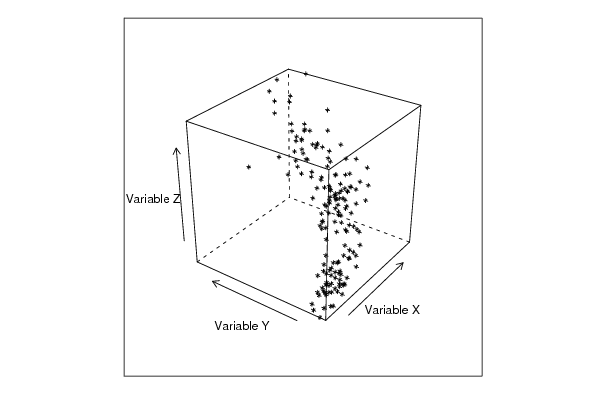
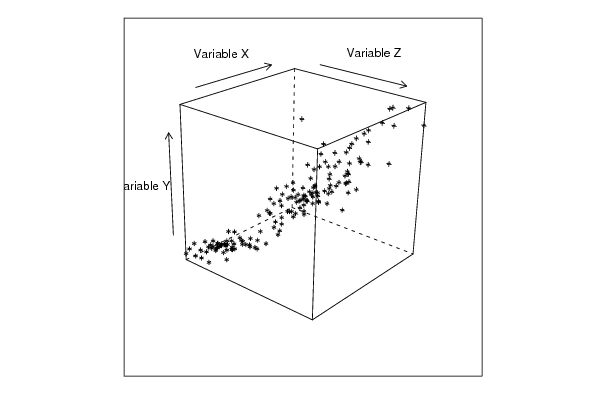
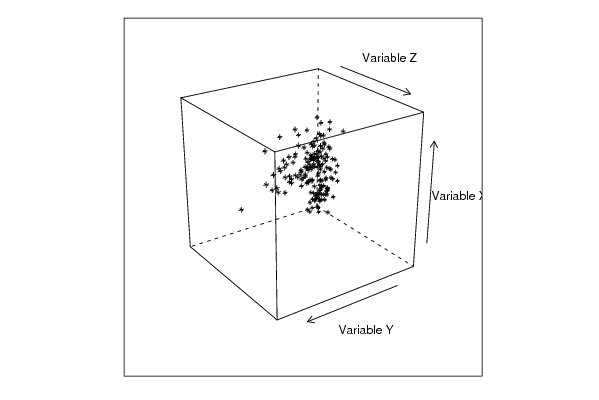
Figures (Output of Computation) | |||||||||||||||||||||
Input Parameters & R Code | |||||||||||||||||||||
| Parameters (Session): | |||||||||||||||||||||
| par1 = 50 ; par2 = 50 ; par3 = Y ; par4 = Y ; par5 = Variable X ; par6 = Variable Y ; par7 = Variable Z ; | |||||||||||||||||||||
| Parameters (R input): | |||||||||||||||||||||
| par1 = 50 ; par2 = 50 ; par3 = Y ; par4 = Y ; par5 = Variable X ; par6 = Variable Y ; par7 = Variable Z ; | |||||||||||||||||||||
| R code (references can be found in the software module): | |||||||||||||||||||||
x <- array(x,dim=c(length(x),1)) | |||||||||||||||||||||