Free Statistics
of Irreproducible Research!
Description of Statistical Computation | |||||||||||||||||||||
|---|---|---|---|---|---|---|---|---|---|---|---|---|---|---|---|---|---|---|---|---|---|
| Author's title | |||||||||||||||||||||
| Author | *The author of this computation has been verified* | ||||||||||||||||||||
| R Software Module | rwasp_cloud.wasp | ||||||||||||||||||||
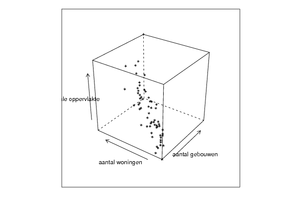
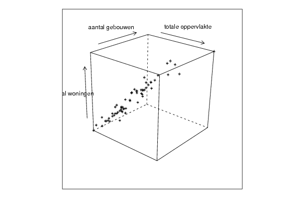
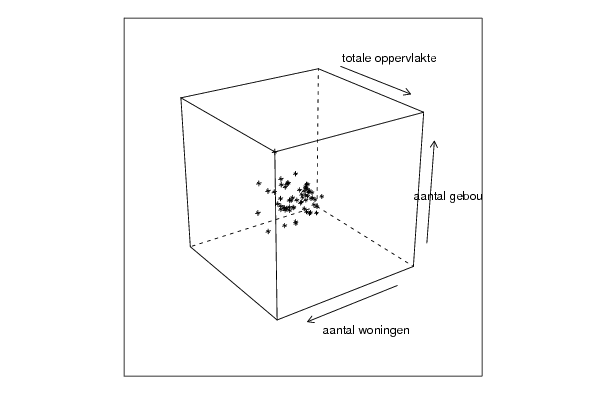
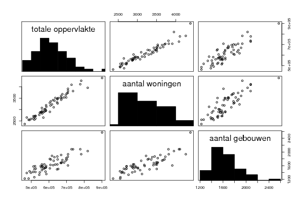
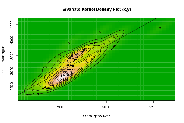
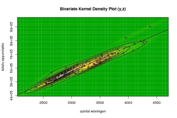
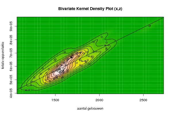
| Title produced by software | Trivariate Scatterplots | ||||||||||||||||||||
| Date of computation | Tue, 11 Nov 2008 12:10:59 -0700 | ||||||||||||||||||||
| Cite this page as follows | Statistical Computations at FreeStatistics.org, Office for Research Development and Education, URL https://freestatistics.org/blog/index.php?v=date/2008/Nov/11/t1226430734b2xu06fhb59duvg.htm/, Retrieved Sun, 19 May 2024 10:11:11 +0000 | ||||||||||||||||||||
| Statistical Computations at FreeStatistics.org, Office for Research Development and Education, URL https://freestatistics.org/blog/index.php?pk=23849, Retrieved Sun, 19 May 2024 10:11:11 +0000 | |||||||||||||||||||||
| QR Codes: | |||||||||||||||||||||
|
| |||||||||||||||||||||
| Original text written by user: | |||||||||||||||||||||
| IsPrivate? | No (this computation is public) | ||||||||||||||||||||
| User-defined keywords | |||||||||||||||||||||
| Estimated Impact | 182 | ||||||||||||||||||||
Tree of Dependent Computations | |||||||||||||||||||||
| Family? (F = Feedback message, R = changed R code, M = changed R Module, P = changed Parameters, D = changed Data) | |||||||||||||||||||||
| - [Bivariate Kernel Density Estimation] [Q1 bivariate dens...] [2008-11-10 13:19:59] [c5a66f1c8528a963efc2b82a8519f117] F D [Bivariate Kernel Density Estimation] [q1 bivariate density] [2008-11-10 14:09:47] [c5a66f1c8528a963efc2b82a8519f117] F RMPD [Partial Correlation] [Q1 partial correl...] [2008-11-10 14:14:55] [c5a66f1c8528a963efc2b82a8519f117] F RMP [Trivariate Scatterplots] [Q1 triviate scatt...] [2008-11-10 14:17:32] [c5a66f1c8528a963efc2b82a8519f117] F [Trivariate Scatterplots] [Q1 - Trivivivivif...] [2008-11-11 19:10:59] [5f3e73ccf1ddc75508eed47fa51813d3] [Current] | |||||||||||||||||||||
| Feedback Forum | |||||||||||||||||||||
Post a new message | |||||||||||||||||||||
Dataset | |||||||||||||||||||||
| Dataseries X: | |||||||||||||||||||||
1515 1510 1225 1577 1417 1224 1693 1633 1639 1914 1586 1552 2081 1500 1437 1470 1849 1387 1592 1589 1798 1935 1887 2027 2080 1556 1682 1785 1869 1781 2082 2570 1862 1936 1504 1765 1607 1577 1493 1615 1700 1335 1523 1623 1540 1637 1524 1419 1821 1593 1357 1263 1750 1405 1393 1639 1679 1551 1744 1429 1784 | |||||||||||||||||||||
| Dataseries Y: | |||||||||||||||||||||
2718 2646 2551 2712 2606 2365 3533 3509 2912 3599 2719 2869 4085 2686 2545 3071 3388 2652 3190 2884 3295 3818 3226 3953 3810 2877 3515 3708 3450 3360 4110 4384 3729 4263 3505 3674 3911 2951 3317 3417 3498 2768 2899 3179 3011 3481 3015 2606 3530 2827 3120 2557 3645 2865 2587 2887 3429 2956 3098 2934 3269 | |||||||||||||||||||||
| Dataseries Z: | |||||||||||||||||||||
524944 568106 484506 512235 523179 462411 685872 635902 573599 668826 520868 555680 727941 516959 489975 559687 630947 473994 583802 553061 604700 708101 617053 819858 736520 567696 666627 701749 647394 610231 777555 901319 707164 782859 652556 676064 707665 561515 645794 623482 673401 544890 605125 608393 579718 647499 575016 510096 697835 561177 584949 516723 695323 548018 497706 559796 669449 583301 626790 580268 649016 | |||||||||||||||||||||
Tables (Output of Computation) | |||||||||||||||||||||
| |||||||||||||||||||||
Figures (Output of Computation) | |||||||||||||||||||||
Input Parameters & R Code | |||||||||||||||||||||
| Parameters (Session): | |||||||||||||||||||||
| par1 = 50 ; par2 = 50 ; par3 = Y ; par4 = Y ; par5 = aantal gebouwen ; par6 = aantal woningen ; par7 = totale oppervlakte ; | |||||||||||||||||||||
| Parameters (R input): | |||||||||||||||||||||
| par1 = 50 ; par2 = 50 ; par3 = Y ; par4 = Y ; par5 = aantal gebouwen ; par6 = aantal woningen ; par7 = totale oppervlakte ; | |||||||||||||||||||||
| R code (references can be found in the software module): | |||||||||||||||||||||
x <- array(x,dim=c(length(x),1)) | |||||||||||||||||||||