Free Statistics
of Irreproducible Research!
Description of Statistical Computation | |||||||||||||||||||||||||||||||||||||
|---|---|---|---|---|---|---|---|---|---|---|---|---|---|---|---|---|---|---|---|---|---|---|---|---|---|---|---|---|---|---|---|---|---|---|---|---|---|
| Author's title | |||||||||||||||||||||||||||||||||||||
| Author | *The author of this computation has been verified* | ||||||||||||||||||||||||||||||||||||
| R Software Module | rwasp_boxcoxnorm.wasp | ||||||||||||||||||||||||||||||||||||
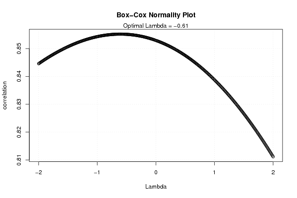
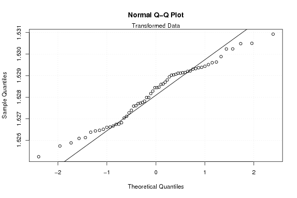
| Title produced by software | Box-Cox Normality Plot | ||||||||||||||||||||||||||||||||||||
| Date of computation | Tue, 11 Nov 2008 10:10:22 -0700 | ||||||||||||||||||||||||||||||||||||
| Cite this page as follows | Statistical Computations at FreeStatistics.org, Office for Research Development and Education, URL https://freestatistics.org/blog/index.php?v=date/2008/Nov/11/t1226423447fz999azvo6zazf4.htm/, Retrieved Sun, 19 May 2024 11:10:35 +0000 | ||||||||||||||||||||||||||||||||||||
| Statistical Computations at FreeStatistics.org, Office for Research Development and Education, URL https://freestatistics.org/blog/index.php?pk=23738, Retrieved Sun, 19 May 2024 11:10:35 +0000 | |||||||||||||||||||||||||||||||||||||
| QR Codes: | |||||||||||||||||||||||||||||||||||||
|
| |||||||||||||||||||||||||||||||||||||
| Original text written by user: | |||||||||||||||||||||||||||||||||||||
| IsPrivate? | No (this computation is public) | ||||||||||||||||||||||||||||||||||||
| User-defined keywords | |||||||||||||||||||||||||||||||||||||
| Estimated Impact | 112 | ||||||||||||||||||||||||||||||||||||
Tree of Dependent Computations | |||||||||||||||||||||||||||||||||||||
| Family? (F = Feedback message, R = changed R code, M = changed R Module, P = changed Parameters, D = changed Data) | |||||||||||||||||||||||||||||||||||||
| - [Box-Cox Normality Plot] [Box cox normality...] [2008-11-11 17:05:37] [3754dd41128068acfc463ebbabce5a9c] - D [Box-Cox Normality Plot] [Box cox normality...] [2008-11-11 17:10:22] [02e7fb326979b65614900650d62c19a6] [Current] - RMPD [Maximum-likelihood Fitting - Normal Distribution] [ML normal distrib...] [2008-11-11 17:15:34] [3754dd41128068acfc463ebbabce5a9c] | |||||||||||||||||||||||||||||||||||||
| Feedback Forum | |||||||||||||||||||||||||||||||||||||
Post a new message | |||||||||||||||||||||||||||||||||||||
Dataset | |||||||||||||||||||||||||||||||||||||
| Dataseries X: | |||||||||||||||||||||||||||||||||||||
2894,3 2838,1 3137,7 2703,7 2623,6 2691,1 2577,9 2430,5 2871 2922,5 2810,8 3070,3 2790 2821 3383,6 3038,4 2877,3 3283,7 2927,3 2952,5 3328,9 3467,3 3355,6 3707 3275,6 3466,5 4054,3 3708,5 3339 3559,8 3189,2 3620,7 3915,4 3804,3 4391,6 4975,9 4478,7 4455,8 5661,8 4062,8 4257,7 4114,2 3793,8 4170 4004,9 4129,7 4116 4133,8 4081,2 3854,1 4239,8 3718,5 4183,1 4336,1 4299,2 4285,3 4676,7 4980,6 5207,4 5221,7 | |||||||||||||||||||||||||||||||||||||
Tables (Output of Computation) | |||||||||||||||||||||||||||||||||||||
| |||||||||||||||||||||||||||||||||||||
Figures (Output of Computation) | |||||||||||||||||||||||||||||||||||||
Input Parameters & R Code | |||||||||||||||||||||||||||||||||||||
| Parameters (Session): | |||||||||||||||||||||||||||||||||||||
| Parameters (R input): | |||||||||||||||||||||||||||||||||||||
| R code (references can be found in the software module): | |||||||||||||||||||||||||||||||||||||
n <- length(x) | |||||||||||||||||||||||||||||||||||||