Free Statistics
of Irreproducible Research!
Description of Statistical Computation | |||||||||||||||||||||||||||||||||||||||||||||
|---|---|---|---|---|---|---|---|---|---|---|---|---|---|---|---|---|---|---|---|---|---|---|---|---|---|---|---|---|---|---|---|---|---|---|---|---|---|---|---|---|---|---|---|---|---|
| Author's title | |||||||||||||||||||||||||||||||||||||||||||||
| Author | *The author of this computation has been verified* | ||||||||||||||||||||||||||||||||||||||||||||
| R Software Module | rwasp_boxcoxlin.wasp | ||||||||||||||||||||||||||||||||||||||||||||
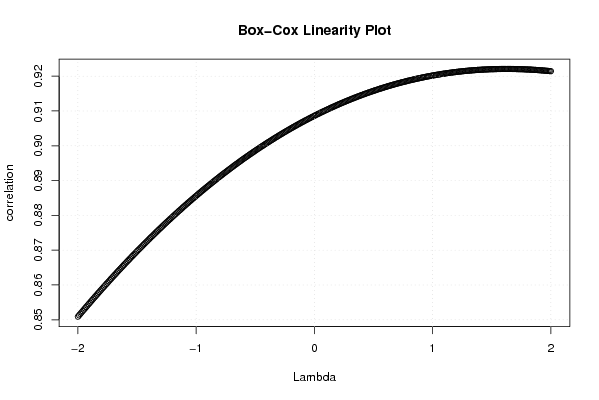
| Title produced by software | Box-Cox Linearity Plot | ||||||||||||||||||||||||||||||||||||||||||||
| Date of computation | Tue, 11 Nov 2008 09:33:36 -0700 | ||||||||||||||||||||||||||||||||||||||||||||
| Cite this page as follows | Statistical Computations at FreeStatistics.org, Office for Research Development and Education, URL https://freestatistics.org/blog/index.php?v=date/2008/Nov/11/t1226421244bgs84rapke3tski.htm/, Retrieved Sun, 19 May 2024 12:13:08 +0000 | ||||||||||||||||||||||||||||||||||||||||||||
| Statistical Computations at FreeStatistics.org, Office for Research Development and Education, URL https://freestatistics.org/blog/index.php?pk=23692, Retrieved Sun, 19 May 2024 12:13:08 +0000 | |||||||||||||||||||||||||||||||||||||||||||||
| QR Codes: | |||||||||||||||||||||||||||||||||||||||||||||
|
| |||||||||||||||||||||||||||||||||||||||||||||
| Original text written by user: | |||||||||||||||||||||||||||||||||||||||||||||
| IsPrivate? | No (this computation is public) | ||||||||||||||||||||||||||||||||||||||||||||
| User-defined keywords | |||||||||||||||||||||||||||||||||||||||||||||
| Estimated Impact | 142 | ||||||||||||||||||||||||||||||||||||||||||||
Tree of Dependent Computations | |||||||||||||||||||||||||||||||||||||||||||||
| Family? (F = Feedback message, R = changed R code, M = changed R Module, P = changed Parameters, D = changed Data) | |||||||||||||||||||||||||||||||||||||||||||||
| F [Box-Cox Linearity Plot] [Various EDA topic...] [2008-11-11 16:33:36] [db9a5fd0f9c3e1245d8075d8bb09236d] [Current] | |||||||||||||||||||||||||||||||||||||||||||||
| Feedback Forum | |||||||||||||||||||||||||||||||||||||||||||||
Post a new message | |||||||||||||||||||||||||||||||||||||||||||||
Dataset | |||||||||||||||||||||||||||||||||||||||||||||
| Dataseries X: | |||||||||||||||||||||||||||||||||||||||||||||
8638,7 11063,7 11855,7 10684,5 11337,4 10478 11123,9 12909,3 11339,9 10462,2 12733,5 10519,2 10414,9 12476,8 12384,6 12266,7 12919,9 11497,3 12142 13919,4 12656,8 12034,1 13199,7 10881,3 11301,2 13643,9 12517 13981,1 14275,7 13435 13565,7 16216,3 12970 14079,9 14235 12213,4 12581 14130,4 14210,8 14378,5 13142,8 13714,7 13621,9 15379,8 13306,3 14391,2 14909,9 14025,4 12951,2 14344,3 16213,3 15544,5 14750,6 17292,7 17568,5 17930,8 18644,7 16694,8 17242,8 16979,9 | |||||||||||||||||||||||||||||||||||||||||||||
| Dataseries Y: | |||||||||||||||||||||||||||||||||||||||||||||
3219,2 3552,3 3787,7 3392,7 3550 3681,9 3519,1 4283,2 4046,2 3824,9 4793,1 3977,7 3983,4 4152,9 4286,1 4348,1 3949,3 4166,7 4217,9 4528,2 4232,2 4470,9 5121,2 4170,8 4398,6 4491,4 4251,8 4901,9 4745,2 4666,9 4210,4 5273,6 4095,3 4610,1 4718,1 4185,5 4314,7 4422,6 5059,2 5043,6 4436,6 4922,6 4454,8 5058,7 4768,9 5171,8 4989,3 5202,1 4838,4 4876,5 5845,3 5686,3 4753,8 6620,4 5597,2 5643,5 6357,3 5909,1 6165,8 6321,6 | |||||||||||||||||||||||||||||||||||||||||||||
Tables (Output of Computation) | |||||||||||||||||||||||||||||||||||||||||||||
| |||||||||||||||||||||||||||||||||||||||||||||
Figures (Output of Computation) | |||||||||||||||||||||||||||||||||||||||||||||
Input Parameters & R Code | |||||||||||||||||||||||||||||||||||||||||||||
| Parameters (Session): | |||||||||||||||||||||||||||||||||||||||||||||
| Parameters (R input): | |||||||||||||||||||||||||||||||||||||||||||||
| R code (references can be found in the software module): | |||||||||||||||||||||||||||||||||||||||||||||
n <- length(x) | |||||||||||||||||||||||||||||||||||||||||||||