Free Statistics
of Irreproducible Research!
Description of Statistical Computation | |||||||||||||||||||||||||||||||||||||||||||||
|---|---|---|---|---|---|---|---|---|---|---|---|---|---|---|---|---|---|---|---|---|---|---|---|---|---|---|---|---|---|---|---|---|---|---|---|---|---|---|---|---|---|---|---|---|---|
| Author's title | |||||||||||||||||||||||||||||||||||||||||||||
| Author | *The author of this computation has been verified* | ||||||||||||||||||||||||||||||||||||||||||||
| R Software Module | rwasp_boxcoxlin.wasp | ||||||||||||||||||||||||||||||||||||||||||||
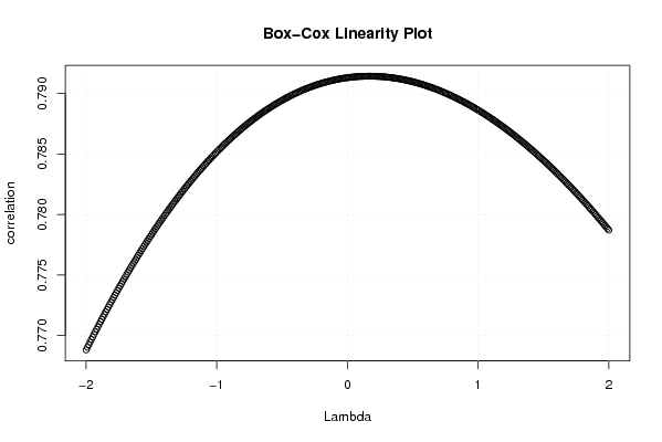
| Title produced by software | Box-Cox Linearity Plot | ||||||||||||||||||||||||||||||||||||||||||||
| Date of computation | Tue, 11 Nov 2008 09:18:23 -0700 | ||||||||||||||||||||||||||||||||||||||||||||
| Cite this page as follows | Statistical Computations at FreeStatistics.org, Office for Research Development and Education, URL https://freestatistics.org/blog/index.php?v=date/2008/Nov/11/t1226420360gp81j6pwbie32ts.htm/, Retrieved Sun, 19 May 2024 08:55:15 +0000 | ||||||||||||||||||||||||||||||||||||||||||||
| Statistical Computations at FreeStatistics.org, Office for Research Development and Education, URL https://freestatistics.org/blog/index.php?pk=23653, Retrieved Sun, 19 May 2024 08:55:15 +0000 | |||||||||||||||||||||||||||||||||||||||||||||
| QR Codes: | |||||||||||||||||||||||||||||||||||||||||||||
|
| |||||||||||||||||||||||||||||||||||||||||||||
| Original text written by user: | |||||||||||||||||||||||||||||||||||||||||||||
| IsPrivate? | No (this computation is public) | ||||||||||||||||||||||||||||||||||||||||||||
| User-defined keywords | |||||||||||||||||||||||||||||||||||||||||||||
| Estimated Impact | 178 | ||||||||||||||||||||||||||||||||||||||||||||
Tree of Dependent Computations | |||||||||||||||||||||||||||||||||||||||||||||
| Family? (F = Feedback message, R = changed R code, M = changed R Module, P = changed Parameters, D = changed Data) | |||||||||||||||||||||||||||||||||||||||||||||
| F [Box-Cox Linearity Plot] [Q3] [2008-11-11 16:15:27] [299afd6311e4c20059ea2f05c8dd029d] F D [Box-Cox Linearity Plot] [Q4] [2008-11-11 16:18:23] [5e2b1e7aa808f9f0d23fd35605d4968f] [Current] F RMPD [Maximum-likelihood Fitting - Normal Distribution] [Q5] [2008-11-11 16:26:11] [299afd6311e4c20059ea2f05c8dd029d] - D [Maximum-likelihood Fitting - Normal Distribution] [Verbetering Q5] [2008-11-23 15:59:00] [299afd6311e4c20059ea2f05c8dd029d] - RMPD [Testing Mean with known Variance - Critical Value] [Q1] [2008-11-11 16:36:56] [299afd6311e4c20059ea2f05c8dd029d] F RMPD [Testing Mean with known Variance - Critical Value] [Q1] [2008-11-11 16:36:56] [299afd6311e4c20059ea2f05c8dd029d] - RMPD [Testing Variance - p-value (probability)] [Q2] [2008-11-11 16:43:10] [299afd6311e4c20059ea2f05c8dd029d] - RM [Testing Mean with known Variance - Critical Value] [Q4] [2008-11-11 17:11:47] [299afd6311e4c20059ea2f05c8dd029d] F RMPD [Testing Mean with known Variance - Type II Error] [Q3] [2008-11-11 17:07:30] [299afd6311e4c20059ea2f05c8dd029d] - [Testing Mean with known Variance - Type II Error] [Q4] [2008-11-11 17:16:18] [299afd6311e4c20059ea2f05c8dd029d] - RM [Testing Mean with known Variance - Critical Value] [Q5] [2008-11-11 17:18:41] [299afd6311e4c20059ea2f05c8dd029d] F RM [Testing Sample Mean with known Variance - Confidence Interval] [Q5] [2008-11-11 17:20:57] [299afd6311e4c20059ea2f05c8dd029d] - P [Testing Sample Mean with known Variance - Confidence Interval] [Q5 - Verbetering] [2008-11-23 17:28:35] [299afd6311e4c20059ea2f05c8dd029d] - RM [Testing Population Mean with known Variance - Confidence Interval] [Q6] [2008-11-11 17:26:50] [299afd6311e4c20059ea2f05c8dd029d] F RM [Testing Sample Mean with known Variance - Confidence Interval] [Q6 - 2 ] [2008-11-11 17:28:02] [299afd6311e4c20059ea2f05c8dd029d] - P [Testing Sample Mean with known Variance - Confidence Interval] [Q6 - Verbetering] [2008-11-23 17:32:27] [299afd6311e4c20059ea2f05c8dd029d] | |||||||||||||||||||||||||||||||||||||||||||||
| Feedback Forum | |||||||||||||||||||||||||||||||||||||||||||||
Post a new message | |||||||||||||||||||||||||||||||||||||||||||||
Dataset | |||||||||||||||||||||||||||||||||||||||||||||
| Dataseries X: | |||||||||||||||||||||||||||||||||||||||||||||
3277.2 3833 2606.3 3643.8 3686.4 3281.6 3669.3 3191.5 3512.7 3970.7 3601.2 3610 4172.1 3956.2 3142.7 3884.3 3892.2 3613 3730.5 3481.3 3649.5 4215.2 4066.6 4196.8 4536.6 4441.6 3548.3 4735.9 4130.6 4356.2 4159.6 3988 4167.8 4902.2 3909.4 4697.6 4308.9 4420.4 3544.2 4433 4479.7 4533.2 4237.5 4207.4 4394 5148.4 4202.2 4682.5 4884.3 5288.9 4505.2 4611.5 5081.1 4523.1 4412.8 4647.4 4778.6 4495.3 4633.5 4360.5 4517.9 | |||||||||||||||||||||||||||||||||||||||||||||
| Dataseries Y: | |||||||||||||||||||||||||||||||||||||||||||||
12192.5 11268.8 9097.4 12639.8 13040.1 11687.3 11191.7 11391.9 11793.1 13933.2 12778.1 11810.3 13698.4 11956.6 10723.8 13938.9 13979.8 13807.4 12973.9 12509.8 12934.1 14908.3 13772.1 13012.6 14049.9 11816.5 11593.2 14466.2 13615.9 14733.9 13880.7 13527.5 13584 16170.2 13260.6 14741.9 15486.5 13154.5 12621.2 15031.6 15452.4 15428 13105.9 14716.8 14180 16202.2 14392.4 15140.6 15960.1 14351.3 13230.2 15202.1 17157.3 16159.1 13405.7 17224.7 17338.4 17370.6 18817.8 16593.2 17979.5 | |||||||||||||||||||||||||||||||||||||||||||||
Tables (Output of Computation) | |||||||||||||||||||||||||||||||||||||||||||||
| |||||||||||||||||||||||||||||||||||||||||||||
Figures (Output of Computation) | |||||||||||||||||||||||||||||||||||||||||||||
Input Parameters & R Code | |||||||||||||||||||||||||||||||||||||||||||||
| Parameters (Session): | |||||||||||||||||||||||||||||||||||||||||||||
| Parameters (R input): | |||||||||||||||||||||||||||||||||||||||||||||
| R code (references can be found in the software module): | |||||||||||||||||||||||||||||||||||||||||||||
n <- length(x) | |||||||||||||||||||||||||||||||||||||||||||||