Free Statistics
of Irreproducible Research!
Description of Statistical Computation | |||||||||||||||||||||||||||||||||||||||
|---|---|---|---|---|---|---|---|---|---|---|---|---|---|---|---|---|---|---|---|---|---|---|---|---|---|---|---|---|---|---|---|---|---|---|---|---|---|---|---|
| Author's title | Maximum-likelihood Normal Distribution Fitting - Aantal inschrjvingen tweed... | ||||||||||||||||||||||||||||||||||||||
| Author | *The author of this computation has been verified* | ||||||||||||||||||||||||||||||||||||||
| R Software Module | rwasp_fitdistrnorm.wasp | ||||||||||||||||||||||||||||||||||||||
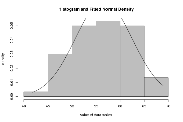
| Title produced by software | Maximum-likelihood Fitting - Normal Distribution | ||||||||||||||||||||||||||||||||||||||
| Date of computation | Tue, 11 Nov 2008 08:33:55 -0700 | ||||||||||||||||||||||||||||||||||||||
| Cite this page as follows | Statistical Computations at FreeStatistics.org, Office for Research Development and Education, URL https://freestatistics.org/blog/index.php?v=date/2008/Nov/11/t1226417752u05tjdnfwgnim2z.htm/, Retrieved Tue, 28 May 2024 07:01:53 +0000 | ||||||||||||||||||||||||||||||||||||||
| Statistical Computations at FreeStatistics.org, Office for Research Development and Education, URL https://freestatistics.org/blog/index.php?pk=23604, Retrieved Tue, 28 May 2024 07:01:53 +0000 | |||||||||||||||||||||||||||||||||||||||
| QR Codes: | |||||||||||||||||||||||||||||||||||||||
|
| |||||||||||||||||||||||||||||||||||||||
| Original text written by user: | |||||||||||||||||||||||||||||||||||||||
| IsPrivate? | No (this computation is public) | ||||||||||||||||||||||||||||||||||||||
| User-defined keywords | |||||||||||||||||||||||||||||||||||||||
| Estimated Impact | 166 | ||||||||||||||||||||||||||||||||||||||
Tree of Dependent Computations | |||||||||||||||||||||||||||||||||||||||
| Family? (F = Feedback message, R = changed R code, M = changed R Module, P = changed Parameters, D = changed Data) | |||||||||||||||||||||||||||||||||||||||
| F [Bivariate Kernel Density Estimation] [Bivariate Kernel ...] [2008-11-10 16:53:50] [819b576fab25b35cfda70f80599828ec] F D [Bivariate Kernel Density Estimation] [Bivaritae Kernel ...] [2008-11-10 16:58:43] [819b576fab25b35cfda70f80599828ec] F RMPD [Partial Correlation] [Partial Correlati...] [2008-11-10 17:08:28] [819b576fab25b35cfda70f80599828ec] - RMPD [Trivariate Scatterplots] [Trivariate Scatte...] [2008-11-10 17:21:24] [819b576fab25b35cfda70f80599828ec] - RMPD [Maximum-likelihood Fitting - Normal Distribution] [Maximum-likelihoo...] [2008-11-10 17:50:35] [819b576fab25b35cfda70f80599828ec] F PD [Maximum-likelihood Fitting - Normal Distribution] [Maximum-likelihoo...] [2008-11-11 15:33:55] [e08fee3874f3333d6b7a377a061b860d] [Current] | |||||||||||||||||||||||||||||||||||||||
| Feedback Forum | |||||||||||||||||||||||||||||||||||||||
Post a new message | |||||||||||||||||||||||||||||||||||||||
Dataset | |||||||||||||||||||||||||||||||||||||||
| Dataseries X: | |||||||||||||||||||||||||||||||||||||||
54.281 63.654 68.918 58.686 67.074 60.183 54.326 54.085 53.564 60.873 53.398 45.164 59.672 56.298 62.361 56.930 62.954 62.431 52.528 54.060 53.093 52.695 52.333 41.747 58.576 57.851 63.721 63.384 61.141 59.231 63.472 49.214 55.816 61.713 48.664 45.351 57.888 54.091 59.098 58.962 55.433 60.403 60.721 48.440 57.981 60.258 47.312 46.980 54.846 56.824 67.744 62.849 54.691 65.461 53.724 54.560 57.722 55.458 48.490 46.362 | |||||||||||||||||||||||||||||||||||||||
Tables (Output of Computation) | |||||||||||||||||||||||||||||||||||||||
| |||||||||||||||||||||||||||||||||||||||
Figures (Output of Computation) | |||||||||||||||||||||||||||||||||||||||
Input Parameters & R Code | |||||||||||||||||||||||||||||||||||||||
| Parameters (Session): | |||||||||||||||||||||||||||||||||||||||
| par1 = 8 ; par2 = 0 ; | |||||||||||||||||||||||||||||||||||||||
| Parameters (R input): | |||||||||||||||||||||||||||||||||||||||
| par1 = 8 ; par2 = 0 ; | |||||||||||||||||||||||||||||||||||||||
| R code (references can be found in the software module): | |||||||||||||||||||||||||||||||||||||||
library(MASS) | |||||||||||||||||||||||||||||||||||||||