Free Statistics
of Irreproducible Research!
Description of Statistical Computation | |||||||||||||||||||||
|---|---|---|---|---|---|---|---|---|---|---|---|---|---|---|---|---|---|---|---|---|---|
| Author's title | |||||||||||||||||||||
| Author | *The author of this computation has been verified* | ||||||||||||||||||||
| R Software Module | rwasp_cloud.wasp | ||||||||||||||||||||
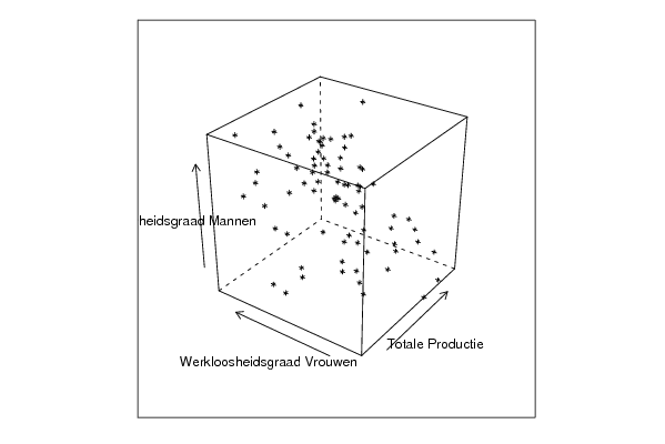
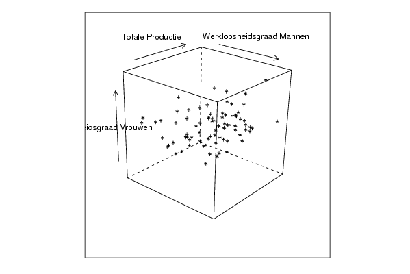
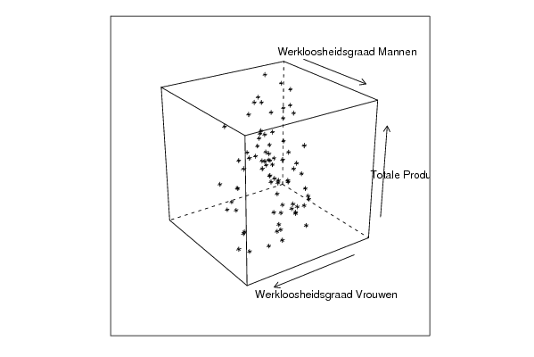
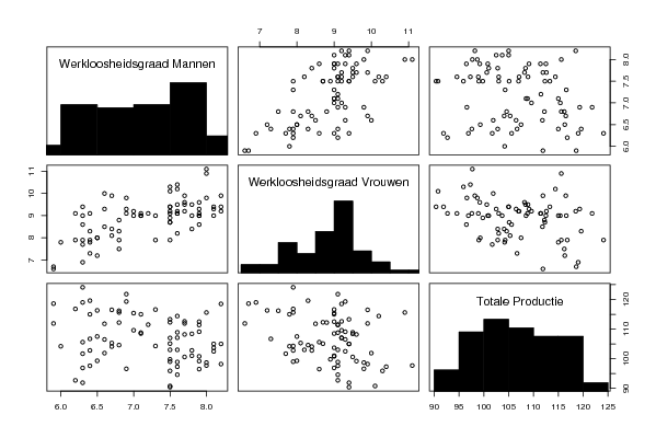
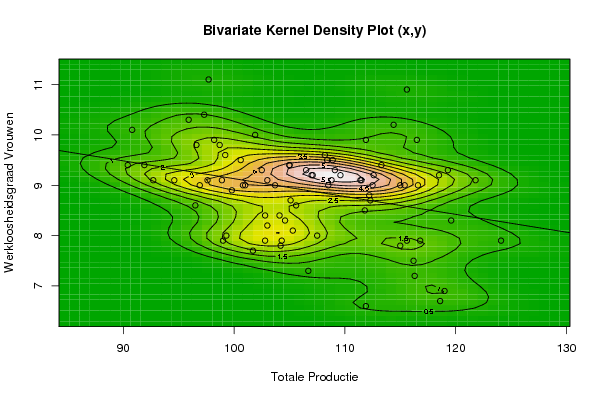
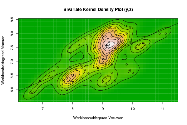
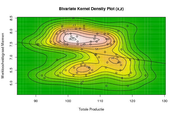
| Title produced by software | Trivariate Scatterplots | ||||||||||||||||||||
| Date of computation | Tue, 11 Nov 2008 08:21:20 -0700 | ||||||||||||||||||||
| Cite this page as follows | Statistical Computations at FreeStatistics.org, Office for Research Development and Education, URL https://freestatistics.org/blog/index.php?v=date/2008/Nov/11/t1226416895k97usapqsg34jtv.htm/, Retrieved Sun, 19 May 2024 10:41:49 +0000 | ||||||||||||||||||||
| Statistical Computations at FreeStatistics.org, Office for Research Development and Education, URL https://freestatistics.org/blog/index.php?pk=23588, Retrieved Sun, 19 May 2024 10:41:49 +0000 | |||||||||||||||||||||
| QR Codes: | |||||||||||||||||||||
|
| |||||||||||||||||||||
| Original text written by user: | |||||||||||||||||||||
| IsPrivate? | No (this computation is public) | ||||||||||||||||||||
| User-defined keywords | |||||||||||||||||||||
| Estimated Impact | 137 | ||||||||||||||||||||
Tree of Dependent Computations | |||||||||||||||||||||
| Family? (F = Feedback message, R = changed R code, M = changed R Module, P = changed Parameters, D = changed Data) | |||||||||||||||||||||
| F [Bivariate Kernel Density Estimation] [] [2008-11-11 15:01:49] [29747f79f5beb5b2516e1271770ecb47] F RMPD [Partial Correlation] [] [2008-11-11 15:17:50] [29747f79f5beb5b2516e1271770ecb47] F RMPD [Trivariate Scatterplots] [] [2008-11-11 15:21:20] [c0a347e3519123f7eef62b705326dad9] [Current] F RMPD [Hierarchical Clustering] [] [2008-11-11 15:27:51] [29747f79f5beb5b2516e1271770ecb47] F RMPD [Box-Cox Linearity Plot] [] [2008-11-11 15:33:03] [29747f79f5beb5b2516e1271770ecb47] F RMPD [Testing Mean with known Variance - Critical Value] [] [2008-11-11 16:11:09] [29747f79f5beb5b2516e1271770ecb47] F RM [Testing Mean with known Variance - p-value] [] [2008-11-11 16:21:44] [29747f79f5beb5b2516e1271770ecb47] F RMP [Testing Mean with known Variance - Type II Error] [] [2008-11-11 16:29:04] [29747f79f5beb5b2516e1271770ecb47] - RMP [Testing Mean with known Variance - Sample Size] [] [2008-11-11 16:34:38] [29747f79f5beb5b2516e1271770ecb47] F [Testing Mean with known Variance - Sample Size] [] [2008-11-11 16:40:41] [29747f79f5beb5b2516e1271770ecb47] F RM [Testing Population Mean with known Variance - Confidence Interval] [] [2008-11-11 17:00:42] [29747f79f5beb5b2516e1271770ecb47] F RM [Testing Sample Mean with known Variance - Confidence Interval] [] [2008-11-11 17:05:19] [29747f79f5beb5b2516e1271770ecb47] | |||||||||||||||||||||
| Feedback Forum | |||||||||||||||||||||
Post a new message | |||||||||||||||||||||
Dataset | |||||||||||||||||||||
| Dataseries X: | |||||||||||||||||||||
97.6 96.9 105.6 102.8 101.7 104.2 92.7 91.9 106.5 112.3 102.8 96.5 101.0 98.9 105.1 103.0 99.0 104.3 94.6 90.4 108.9 111.4 100.8 102.5 98.2 98.7 113.3 104.6 99.3 111.8 97.3 97.7 115.6 111.9 107.0 107.1 100.6 99.2 108.4 103.0 99.8 115.0 90.8 95.9 114.4 108.2 112.6 109.1 105.0 105.0 118.5 103.7 112.5 116.6 96.6 101.9 116.5 119.3 115.4 108.5 111.5 108.8 121.8 109.6 112.2 119.6 104.1 105.3 115.0 124.1 116.8 107.5 115.6 116.2 116.3 119.0 111.9 118.6 106.7 | |||||||||||||||||||||
| Dataseries Y: | |||||||||||||||||||||
9.1 9.0 8.6 7.9 7.7 7.8 9.1 9.4 9.3 8.7 8.4 8.6 9.0 9.1 8.7 8.2 7.9 7.9 9.1 9.4 9.5 9.1 9.0 9.3 9.9 9.8 9.4 8.3 8.0 8.5 10.4 11.1 10.9 9.9 9.2 9.2 9.5 9.6 9.5 9.1 8.9 9.0 10.1 10.3 10.2 9.6 9.2 9.3 9.4 9.4 9.2 9.0 9.0 9.0 9.8 10.0 9.9 9.3 9.0 9.0 9.1 9.1 9.1 9.2 8.8 8.3 8.4 8.1 7.8 7.9 7.9 8.0 7.9 7.5 7.2 6.9 6.6 6.7 7.3 | |||||||||||||||||||||
| Dataseries Z: | |||||||||||||||||||||
6.4 6.3 6.3 6.4 6.3 6.0 6.2 6.3 6.6 7.5 7.8 7.9 7.8 7.6 7.5 7.6 7.5 7.3 7.6 7.5 7.6 7.9 7.9 8.1 8.2 8.0 7.5 6.8 6.5 6.6 7.6 8.0 8.0 7.7 7.5 7.6 7.7 7.9 7.8 7.5 7.5 7.1 7.5 7.5 7.6 7.7 7.7 7.9 8.1 8.2 8.2 8.1 7.9 7.3 6.9 6.6 6.7 6.9 7.0 7.1 7.2 7.1 6.9 7.0 6.8 6.4 6.7 6.7 6.4 6.3 6.2 6.5 6.8 6.8 6.5 6.3 5.9 5.9 6.4 | |||||||||||||||||||||
Tables (Output of Computation) | |||||||||||||||||||||
| |||||||||||||||||||||
Figures (Output of Computation) | |||||||||||||||||||||
Input Parameters & R Code | |||||||||||||||||||||
| Parameters (Session): | |||||||||||||||||||||
| par1 = 50 ; par2 = 50 ; par3 = Y ; par4 = Y ; par5 = Totale Productie ; par6 = Werkloosheidsgraad Vrouwen ; par7 = Werkloosheidsgraad Mannen ; | |||||||||||||||||||||
| Parameters (R input): | |||||||||||||||||||||
| par1 = 50 ; par2 = 50 ; par3 = Y ; par4 = Y ; par5 = Totale Productie ; par6 = Werkloosheidsgraad Vrouwen ; par7 = Werkloosheidsgraad Mannen ; | |||||||||||||||||||||
| R code (references can be found in the software module): | |||||||||||||||||||||
x <- array(x,dim=c(length(x),1)) | |||||||||||||||||||||