Free Statistics
of Irreproducible Research!
Description of Statistical Computation | |||||||||||||||||||||||||||||||||||||
|---|---|---|---|---|---|---|---|---|---|---|---|---|---|---|---|---|---|---|---|---|---|---|---|---|---|---|---|---|---|---|---|---|---|---|---|---|---|
| Author's title | |||||||||||||||||||||||||||||||||||||
| Author | *The author of this computation has been verified* | ||||||||||||||||||||||||||||||||||||
| R Software Module | rwasp_boxcoxnorm.wasp | ||||||||||||||||||||||||||||||||||||
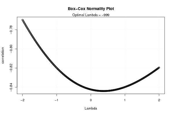
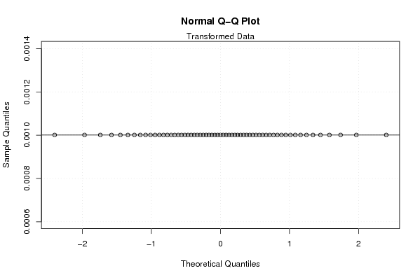
| Title produced by software | Box-Cox Normality Plot | ||||||||||||||||||||||||||||||||||||
| Date of computation | Tue, 11 Nov 2008 07:44:37 -0700 | ||||||||||||||||||||||||||||||||||||
| Cite this page as follows | Statistical Computations at FreeStatistics.org, Office for Research Development and Education, URL https://freestatistics.org/blog/index.php?v=date/2008/Nov/11/t1226414772lcbir8d82dvelez.htm/, Retrieved Sun, 19 May 2024 12:17:40 +0000 | ||||||||||||||||||||||||||||||||||||
| Statistical Computations at FreeStatistics.org, Office for Research Development and Education, URL https://freestatistics.org/blog/index.php?pk=23548, Retrieved Sun, 19 May 2024 12:17:40 +0000 | |||||||||||||||||||||||||||||||||||||
| QR Codes: | |||||||||||||||||||||||||||||||||||||
|
| |||||||||||||||||||||||||||||||||||||
| Original text written by user: | |||||||||||||||||||||||||||||||||||||
| IsPrivate? | No (this computation is public) | ||||||||||||||||||||||||||||||||||||
| User-defined keywords | |||||||||||||||||||||||||||||||||||||
| Estimated Impact | 172 | ||||||||||||||||||||||||||||||||||||
Tree of Dependent Computations | |||||||||||||||||||||||||||||||||||||
| Family? (F = Feedback message, R = changed R code, M = changed R Module, P = changed Parameters, D = changed Data) | |||||||||||||||||||||||||||||||||||||
| - [Box-Cox Linearity Plot] [Box-Cox] [2008-11-11 14:29:04] [adb6b6905cde49db36d59ca44433140d] - RM D [Box-Cox Normality Plot] [Box-Cox Normality...] [2008-11-11 14:44:37] [6d5cd2fe15d123a10639b4bf141c23b5] [Current] F D [Box-Cox Normality Plot] [Box-Cox Normality...] [2008-11-11 23:46:30] [b591abfa820a394aeb0c5ebd9cfa1091] F RMPD [Maximum-likelihood Fitting - Normal Distribution] [Normal Distribution ] [2008-11-12 15:48:53] [b478325fa744e3f2fc16a7222294469c] F D [Maximum-likelihood Fitting - Normal Distribution] [Opdracht3_Q5] [2008-11-12 15:58:44] [3f66c6f083b1153972739491b89fa2dd] F PD [Maximum-likelihood Fitting - Normal Distribution] [task 8 maximum li...] [2008-11-12 20:17:58] [1eab65e90adf64584b8e6f0da23ff414] - RMPD [Univariate Data Series] [Paper 4.2.1] [2008-12-18 18:27:01] [1eab65e90adf64584b8e6f0da23ff414] - RMPD [Histogram] [4.2.1] [2008-12-18 18:38:08] [1eab65e90adf64584b8e6f0da23ff414] - PD [Maximum-likelihood Fitting - Normal Distribution] [4.2.1] [2008-12-18 18:48:23] [1eab65e90adf64584b8e6f0da23ff414] - RMPD [Box-Cox Normality Plot] [4.2.1] [2008-12-18 18:51:19] [1eab65e90adf64584b8e6f0da23ff414] - RMP [Standard Deviation-Mean Plot] [4.2.2] [2008-12-19 10:25:45] [1eab65e90adf64584b8e6f0da23ff414] - RMP [Variance Reduction Matrix] [4.2.2 variantie rdm] [2008-12-19 10:48:41] [1eab65e90adf64584b8e6f0da23ff414] - RMP [(Partial) Autocorrelation Function] [4.2.2] [2008-12-19 10:57:29] [1eab65e90adf64584b8e6f0da23ff414] - P [(Partial) Autocorrelation Function] [4.2.2 D1] [2008-12-19 14:00:41] [1eab65e90adf64584b8e6f0da23ff414] - RMP [Spectral Analysis] [4.2.2 spect] [2008-12-19 14:09:27] [1eab65e90adf64584b8e6f0da23ff414] - RMP [Spectral Analysis] [4.2.2 spec 1] [2008-12-19 14:13:18] [1eab65e90adf64584b8e6f0da23ff414] - RMP [ARIMA Backward Selection] [4.3] [2008-12-19 14:24:21] [1eab65e90adf64584b8e6f0da23ff414] - RMP [(Partial) Autocorrelation Function] [4.2.2] [2008-12-19 17:44:20] [1eab65e90adf64584b8e6f0da23ff414] - RMP [(Partial) Autocorrelation Function] [4.2.2 cor] [2008-12-19 17:50:05] [1eab65e90adf64584b8e6f0da23ff414] - RMP [ARIMA Forecasting] [4.3] [2008-12-19 18:01:56] [1eab65e90adf64584b8e6f0da23ff414] - PD [(Partial) Autocorrelation Function] [4.2.2 pacf] [2008-12-19 16:27:58] [1eab65e90adf64584b8e6f0da23ff414] F D [Box-Cox Normality Plot] [box cox normal plot2] [2008-11-13 08:41:37] [3b5d63cebdc58ed6c519cdb5b6a36d46] | |||||||||||||||||||||||||||||||||||||
| Feedback Forum | |||||||||||||||||||||||||||||||||||||
Post a new message | |||||||||||||||||||||||||||||||||||||
Dataset | |||||||||||||||||||||||||||||||||||||
| Dataseries X: | |||||||||||||||||||||||||||||||||||||
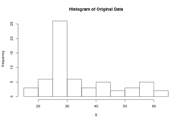
57,42 56,12 59,15 63,77 63,96 57,81 55,3 51,8 53,26 53,38 45,85 44,23 40,22 44,61 49,14 42,94 41,84 37,75 35,54 37,13 33,19 32,67 30,52 30,7 29,59 28,76 29,08 26,95 29,58 28,24 27,28 25,48 24,87 29,87 32,33 30,23 27,46 24,46 27,34 28,37 26,09 25,59 24,67 25,61 25,97 24,31 20,36 19,82 19,32 19,2 21,74 26,29 25,9 25,36 27,64 28,57 25,38 25,71 27,6 25,85 26,54 | |||||||||||||||||||||||||||||||||||||
Tables (Output of Computation) | |||||||||||||||||||||||||||||||||||||
| |||||||||||||||||||||||||||||||||||||
Figures (Output of Computation) | |||||||||||||||||||||||||||||||||||||
Input Parameters & R Code | |||||||||||||||||||||||||||||||||||||
| Parameters (Session): | |||||||||||||||||||||||||||||||||||||
| Parameters (R input): | |||||||||||||||||||||||||||||||||||||
| R code (references can be found in the software module): | |||||||||||||||||||||||||||||||||||||
n <- length(x) | |||||||||||||||||||||||||||||||||||||