Free Statistics
of Irreproducible Research!
Description of Statistical Computation | |||||||||||||||||||||||||||||||||||||||||||||
|---|---|---|---|---|---|---|---|---|---|---|---|---|---|---|---|---|---|---|---|---|---|---|---|---|---|---|---|---|---|---|---|---|---|---|---|---|---|---|---|---|---|---|---|---|---|
| Author's title | |||||||||||||||||||||||||||||||||||||||||||||
| Author | *The author of this computation has been verified* | ||||||||||||||||||||||||||||||||||||||||||||
| R Software Module | rwasp_boxcoxlin.wasp | ||||||||||||||||||||||||||||||||||||||||||||
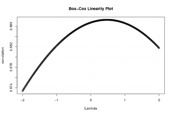
| Title produced by software | Box-Cox Linearity Plot | ||||||||||||||||||||||||||||||||||||||||||||
| Date of computation | Tue, 11 Nov 2008 07:29:04 -0700 | ||||||||||||||||||||||||||||||||||||||||||||
| Cite this page as follows | Statistical Computations at FreeStatistics.org, Office for Research Development and Education, URL https://freestatistics.org/blog/index.php?v=date/2008/Nov/11/t1226413984s6sjpoe0v2jc0g1.htm/, Retrieved Sun, 19 May 2024 10:20:52 +0000 | ||||||||||||||||||||||||||||||||||||||||||||
| Statistical Computations at FreeStatistics.org, Office for Research Development and Education, URL https://freestatistics.org/blog/index.php?pk=23532, Retrieved Sun, 19 May 2024 10:20:52 +0000 | |||||||||||||||||||||||||||||||||||||||||||||
| QR Codes: | |||||||||||||||||||||||||||||||||||||||||||||
|
| |||||||||||||||||||||||||||||||||||||||||||||
| Original text written by user: | |||||||||||||||||||||||||||||||||||||||||||||
| IsPrivate? | No (this computation is public) | ||||||||||||||||||||||||||||||||||||||||||||
| User-defined keywords | |||||||||||||||||||||||||||||||||||||||||||||
| Estimated Impact | 171 | ||||||||||||||||||||||||||||||||||||||||||||
Tree of Dependent Computations | |||||||||||||||||||||||||||||||||||||||||||||
| Family? (F = Feedback message, R = changed R code, M = changed R Module, P = changed Parameters, D = changed Data) | |||||||||||||||||||||||||||||||||||||||||||||
| - [Box-Cox Linearity Plot] [Box-Cox] [2008-11-11 14:29:04] [6d5cd2fe15d123a10639b4bf141c23b5] [Current] - RM D [Box-Cox Normality Plot] [Box-Cox Normality...] [2008-11-11 14:44:37] [adb6b6905cde49db36d59ca44433140d] F D [Box-Cox Normality Plot] [Box-Cox Normality...] [2008-11-11 23:46:30] [b591abfa820a394aeb0c5ebd9cfa1091] F RMPD [Maximum-likelihood Fitting - Normal Distribution] [Normal Distribution ] [2008-11-12 15:48:53] [b478325fa744e3f2fc16a7222294469c] F D [Maximum-likelihood Fitting - Normal Distribution] [Opdracht3_Q5] [2008-11-12 15:58:44] [3f66c6f083b1153972739491b89fa2dd] F PD [Maximum-likelihood Fitting - Normal Distribution] [task 8 maximum li...] [2008-11-12 20:17:58] [1eab65e90adf64584b8e6f0da23ff414] - RMPD [Univariate Data Series] [Paper 4.2.1] [2008-12-18 18:27:01] [1eab65e90adf64584b8e6f0da23ff414] - RMPD [Histogram] [4.2.1] [2008-12-18 18:38:08] [1eab65e90adf64584b8e6f0da23ff414] - PD [Maximum-likelihood Fitting - Normal Distribution] [4.2.1] [2008-12-18 18:48:23] [1eab65e90adf64584b8e6f0da23ff414] - RMPD [Box-Cox Normality Plot] [4.2.1] [2008-12-18 18:51:19] [1eab65e90adf64584b8e6f0da23ff414] - RMP [Standard Deviation-Mean Plot] [4.2.2] [2008-12-19 10:25:45] [1eab65e90adf64584b8e6f0da23ff414] - RMP [Variance Reduction Matrix] [4.2.2 variantie rdm] [2008-12-19 10:48:41] [1eab65e90adf64584b8e6f0da23ff414] - RMP [(Partial) Autocorrelation Function] [4.2.2] [2008-12-19 10:57:29] [1eab65e90adf64584b8e6f0da23ff414] - P [(Partial) Autocorrelation Function] [4.2.2 D1] [2008-12-19 14:00:41] [1eab65e90adf64584b8e6f0da23ff414] - RMP [Spectral Analysis] [4.2.2 spect] [2008-12-19 14:09:27] [1eab65e90adf64584b8e6f0da23ff414] - RMP [Spectral Analysis] [4.2.2 spec 1] [2008-12-19 14:13:18] [1eab65e90adf64584b8e6f0da23ff414] - RMP [ARIMA Backward Selection] [4.3] [2008-12-19 14:24:21] [1eab65e90adf64584b8e6f0da23ff414] - RMP [(Partial) Autocorrelation Function] [4.2.2] [2008-12-19 17:44:20] [1eab65e90adf64584b8e6f0da23ff414] - RMP [(Partial) Autocorrelation Function] [4.2.2 cor] [2008-12-19 17:50:05] [1eab65e90adf64584b8e6f0da23ff414] - RMP [ARIMA Forecasting] [4.3] [2008-12-19 18:01:56] [1eab65e90adf64584b8e6f0da23ff414] - PD [(Partial) Autocorrelation Function] [4.2.2 pacf] [2008-12-19 16:27:58] [1eab65e90adf64584b8e6f0da23ff414] F D [Box-Cox Normality Plot] [box cox normal plot2] [2008-11-13 08:41:37] [3b5d63cebdc58ed6c519cdb5b6a36d46] F RMPD [Maximum-likelihood Fitting - Normal Distribution] [Maximum likehood ...] [2008-11-11 15:10:16] [adb6b6905cde49db36d59ca44433140d] F D [Maximum-likelihood Fitting - Normal Distribution] [Maximum-likelihoo...] [2008-11-11 23:51:03] [b591abfa820a394aeb0c5ebd9cfa1091] F D [Maximum-likelihood Fitting - Normal Distribution] [normal distribution] [2008-11-13 08:47:07] [3b5d63cebdc58ed6c519cdb5b6a36d46] | |||||||||||||||||||||||||||||||||||||||||||||
| Feedback Forum | |||||||||||||||||||||||||||||||||||||||||||||
Post a new message | |||||||||||||||||||||||||||||||||||||||||||||
Dataset | |||||||||||||||||||||||||||||||||||||||||||||
| Dataseries X: | |||||||||||||||||||||||||||||||||||||||||||||
13812 13031 12574 11964 11451 11346 11353 10702 10646 10556 10463 10407 10625 10872 10805 10653 10574 10431 10383 10296 10872 10635 10297 10570 10662 10709 10413 10846 10371 9924 9828 9897 9721 10171 10738 10812 10511 10244 10368 10457 10186 10166 10827 10997 10940 10756 10893 10236 9960 10018 10063 10002 9728 10002 10177 9948 9394 9308 9155 9103 9732 | |||||||||||||||||||||||||||||||||||||||||||||
| Dataseries Y: | |||||||||||||||||||||||||||||||||||||||||||||
57.42 56.12 59.15 63.77 63.96 57.81 55.3 51.8 53.26 53.38 45.85 44.23 40.22 44.61 49.14 42.94 41.84 37.75 35.54 37.13 33.19 32.67 30.52 30.7 29.59 28.76 29.08 26.95 29.58 28.24 27.28 25.48 24.87 29.87 32.33 30.23 27.46 24.46 27.34 28.37 26.09 25.59 24.67 25.61 25.97 24.31 20.36 19.82 19.32 19.2 21.74 26.29 25.9 25.36 27.64 28.57 25.38 25.71 27.6 25.85 26.54 | |||||||||||||||||||||||||||||||||||||||||||||
Tables (Output of Computation) | |||||||||||||||||||||||||||||||||||||||||||||
| |||||||||||||||||||||||||||||||||||||||||||||
Figures (Output of Computation) | |||||||||||||||||||||||||||||||||||||||||||||
Input Parameters & R Code | |||||||||||||||||||||||||||||||||||||||||||||
| Parameters (Session): | |||||||||||||||||||||||||||||||||||||||||||||
| Parameters (R input): | |||||||||||||||||||||||||||||||||||||||||||||
| R code (references can be found in the software module): | |||||||||||||||||||||||||||||||||||||||||||||
n <- length(x) | |||||||||||||||||||||||||||||||||||||||||||||