Free Statistics
of Irreproducible Research!
Description of Statistical Computation | |||||||||||||||||||||
|---|---|---|---|---|---|---|---|---|---|---|---|---|---|---|---|---|---|---|---|---|---|
| Author's title | |||||||||||||||||||||
| Author | *The author of this computation has been verified* | ||||||||||||||||||||
| R Software Module | rwasp_cloud.wasp | ||||||||||||||||||||
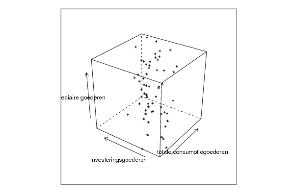
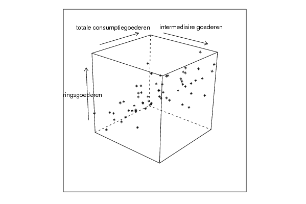
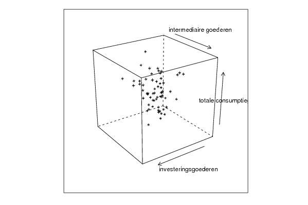
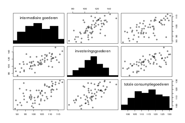
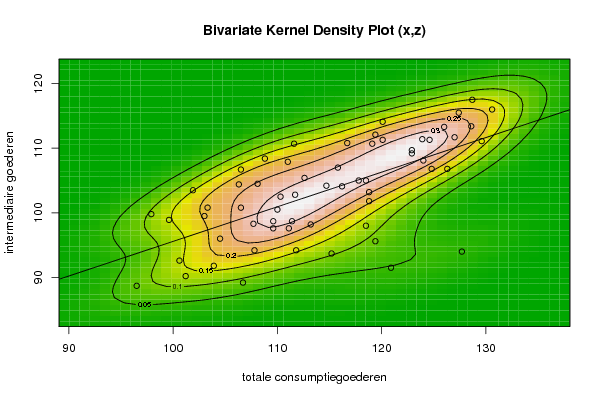
| Title produced by software | Trivariate Scatterplots | ||||||||||||||||||||
| Date of computation | Tue, 11 Nov 2008 07:27:56 -0700 | ||||||||||||||||||||
| Cite this page as follows | Statistical Computations at FreeStatistics.org, Office for Research Development and Education, URL https://freestatistics.org/blog/index.php?v=date/2008/Nov/11/t12264137202spknqvg0u3lhzm.htm/, Retrieved Sun, 19 May 2024 10:41:21 +0000 | ||||||||||||||||||||
| Statistical Computations at FreeStatistics.org, Office for Research Development and Education, URL https://freestatistics.org/blog/index.php?pk=23523, Retrieved Sun, 19 May 2024 10:41:21 +0000 | |||||||||||||||||||||
| QR Codes: | |||||||||||||||||||||
|
| |||||||||||||||||||||
| Original text written by user: | |||||||||||||||||||||
| IsPrivate? | No (this computation is public) | ||||||||||||||||||||
| User-defined keywords | |||||||||||||||||||||
| Estimated Impact | 144 | ||||||||||||||||||||
Tree of Dependent Computations | |||||||||||||||||||||
| Family? (F = Feedback message, R = changed R code, M = changed R Module, P = changed Parameters, D = changed Data) | |||||||||||||||||||||
| F [Bivariate Kernel Density Estimation] [Q1] [2008-11-11 14:12:08] [491a70d26f8c977398d8a0c1c87d3dd4] F RMPD [Partial Correlation] [Q2] [2008-11-11 14:20:55] [491a70d26f8c977398d8a0c1c87d3dd4] F RMP [Trivariate Scatterplots] [Q1] [2008-11-11 14:27:56] [2ba2a74112fb2c960057a572bf2825d3] [Current] | |||||||||||||||||||||
| Feedback Forum | |||||||||||||||||||||
Post a new message | |||||||||||||||||||||
Dataset | |||||||||||||||||||||
| Dataseries X: | |||||||||||||||||||||
109.6 103 111.6 106.3 97.9 108.8 103.9 101.2 122.9 123.9 111.7 120.9 99.6 103.3 119.4 106.5 101.9 124.6 106.5 107.8 127.4 120.1 118.5 127.7 107.7 104.5 118.8 110.3 109.6 119.1 96.5 106.7 126.3 116.2 118.8 115.2 110 111.4 129.6 108.1 117.8 122.9 100.6 111.8 127 128.6 124.8 118.5 114.7 112.6 128.7 111 115.8 126 111.1 113.2 120.1 130.6 124 119.4 116.7 | |||||||||||||||||||||
| Dataseries Y: | |||||||||||||||||||||
93.4 101.1 114.2 104.8 113.3 118.2 83.6 73.9 99.5 97.7 103 106.3 92.2 101.8 122.8 111.8 106.3 121.5 81.9 85.4 110.9 117.3 106.3 105.6 101.2 105.9 126.3 111.9 108.9 127.2 94.2 85.7 116.2 107.2 110.5 112 104.4 112 132.8 110.8 128.7 136.8 94.8 88.8 123.2 125.3 122.7 125.8 116.3 118.6 142.1 127.9 132 152.4 110.8 99.1 134.9 133.2 131 133.9 119.9 | |||||||||||||||||||||
| Dataseries Z: | |||||||||||||||||||||
97.6 99.5 110.7 104.4 99.8 108.4 91.8 90.2 109.2 111.4 102.8 91.5 98.9 100.8 112.1 106.7 103.5 111.3 100.8 94.2 115.5 114.1 105 94 98.3 96 101.8 102.5 98.7 110.7 88.7 89.2 106.8 104.1 103.2 93.7 100.5 98.7 111.1 104.5 105 109.7 92.6 94.2 111.7 113.4 106.8 98 104.2 105.4 117.5 107.9 107 113.3 97.6 98.2 111.3 116 108.1 95.6 110.8 | |||||||||||||||||||||
Tables (Output of Computation) | |||||||||||||||||||||
| |||||||||||||||||||||
Figures (Output of Computation) | |||||||||||||||||||||
Input Parameters & R Code | |||||||||||||||||||||
| Parameters (Session): | |||||||||||||||||||||
| par1 = 50 ; par2 = 50 ; par3 = Y ; par4 = Y ; par5 = totale consumptiegoederen ; par6 = investeringsgoederen ; par7 = intermediaire goederen ; | |||||||||||||||||||||
| Parameters (R input): | |||||||||||||||||||||
| par1 = 50 ; par2 = 50 ; par3 = Y ; par4 = Y ; par5 = totale consumptiegoederen ; par6 = investeringsgoederen ; par7 = intermediaire goederen ; | |||||||||||||||||||||
| R code (references can be found in the software module): | |||||||||||||||||||||
x <- array(x,dim=c(length(x),1)) | |||||||||||||||||||||