Free Statistics
of Irreproducible Research!
Description of Statistical Computation | |||||||||||||||||||||
|---|---|---|---|---|---|---|---|---|---|---|---|---|---|---|---|---|---|---|---|---|---|
| Author's title | |||||||||||||||||||||
| Author | *The author of this computation has been verified* | ||||||||||||||||||||
| R Software Module | rwasp_cloud.wasp | ||||||||||||||||||||
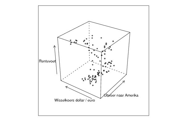
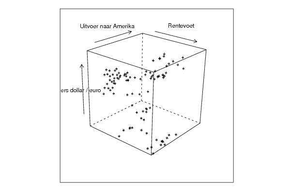
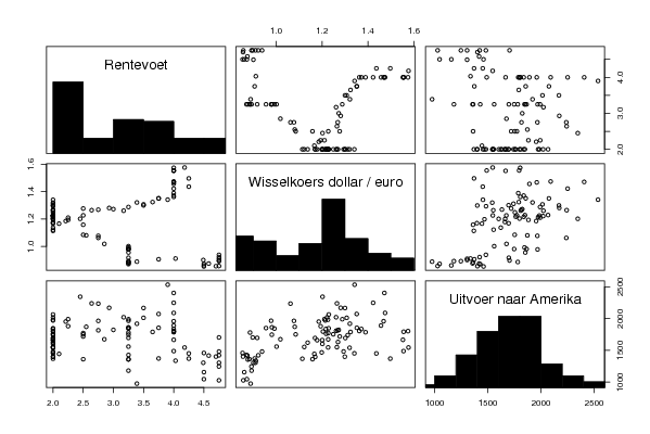
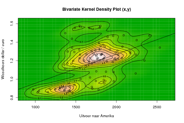
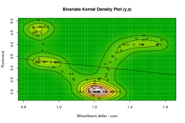
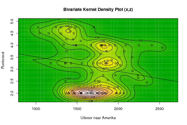
| Title produced by software | Trivariate Scatterplots | ||||||||||||||||||||
| Date of computation | Tue, 11 Nov 2008 06:08:21 -0700 | ||||||||||||||||||||
| Cite this page as follows | Statistical Computations at FreeStatistics.org, Office for Research Development and Education, URL https://freestatistics.org/blog/index.php?v=date/2008/Nov/11/t1226408933fdjr1a6n5dr9slq.htm/, Retrieved Sun, 19 May 2024 08:50:52 +0000 | ||||||||||||||||||||
| Statistical Computations at FreeStatistics.org, Office for Research Development and Education, URL https://freestatistics.org/blog/index.php?pk=23439, Retrieved Sun, 19 May 2024 08:50:52 +0000 | |||||||||||||||||||||
| QR Codes: | |||||||||||||||||||||
|
| |||||||||||||||||||||
| Original text written by user: | |||||||||||||||||||||
| IsPrivate? | No (this computation is public) | ||||||||||||||||||||
| User-defined keywords | |||||||||||||||||||||
| Estimated Impact | 117 | ||||||||||||||||||||
Tree of Dependent Computations | |||||||||||||||||||||
| Family? (F = Feedback message, R = changed R code, M = changed R Module, P = changed Parameters, D = changed Data) | |||||||||||||||||||||
| - [Trivariate Scatterplots] [Various EDA Topic...] [2008-11-11 13:08:21] [620b6ad5c4696049e39cb73ce029682c] [Current] | |||||||||||||||||||||
| Feedback Forum | |||||||||||||||||||||
Post a new message | |||||||||||||||||||||
Dataset | |||||||||||||||||||||
| Dataseries X: | |||||||||||||||||||||
1045.9 1401.9 1027.6 1703.8 1481.3 1422.7 1304.7 1246.1 1417.8 1459.1 1156.4 1304.5 1336.9 1372.3 975.5 1180.8 1361.3 1428.1 1355.9 1781.2 1697 1852 1844.1 1967.2 1747.1 1863.9 1559.3 1675 2237.5 1965.2 1871.5 1752.2 1360.7 1444.3 1621.6 1368 1553.9 1695.3 1397.1 1848.4 1809.2 1551.1 1546.6 1467.9 1662.4 1972.3 1673.5 1762 2019.8 1754.3 1400.4 1453.6 1740.9 1694.6 1541.2 1482.3 1632.1 1837.3 1797 2066.2 1983.8 1601.7 1660.3 1954 1991.9 1881.4 2345.5 1773.1 1719.2 2240.9 1816.4 2171.3 1823.3 2022.5 1991 1920 2168.4 2013.5 1790.8 1855.7 2074 2535.8 1837.2 1805.1 1785.7 2250 1959.7 1890.8 2405.7 2090.3 1666.5 1803.5 1793.8 1488.8 1545 1369.9 1451.6 | |||||||||||||||||||||
| Dataseries Y: | |||||||||||||||||||||
0,8721 0,8552 0,8564 0,8973 0,9383 0,9217 0,9095 0,892 0,8742 0,8532 0,8607 0,9005 0,9111 0,9059 0,8883 0,8924 0,8833 0,87 0,8758 0,8858 0,917 0,9554 0,9922 0,9778 0,9808 0,9811 1,0014 1,0183 1,0622 1,0773 1,0807 1,0848 1,1582 1,1663 1,1372 1,1139 1,1222 1,1692 1,1702 1,2286 1,2613 1,2646 1,2262 1,1985 1,2007 1,2138 1,2266 1,2176 1,2218 1,249 1,2991 1,3408 1,3119 1,3014 1,3201 1,2938 1,2694 1,2165 1,2037 1,2292 1,2256 1,2015 1,1786 1,1856 1,2103 1,1938 1,202 1,2271 1,277 1,265 1,2684 1,2811 1,2727 1,2611 1,2881 1,3213 1,2999 1,3074 1,3242 1,3516 1,3511 1,3419 1,3716 1,3622 1,3896 1,4227 1,4684 1,457 1,4718 1,4748 1,5527 1,575 1,5557 1,5553 1,577 1,4975 1,4369 | |||||||||||||||||||||
| Dataseries Z: | |||||||||||||||||||||
4.5 4.7 4.75 4.75 4.75 4.75 4.75 4.75 4.58 4.5 4.5 4.49 4.03 3.75 3.39 3.25 3.25 3.25 3.25 3.25 3.25 3.25 3.25 3.25 3.25 3.25 3.25 2.85 2.75 2.75 2.55 2.5 2.5 2.1 2 2 2 2 2 2 2 2 2 2 2 2 2 2 2 2 2 2 2 2 2 2 2 2 2 2 2 2 2 2.21 2.25 2.25 2.45 2.5 2.5 2.64 2.75 2.93 3 3.17 3.25 3.39 3.5 3.5 3.65 3.75 3.75 3.9 4 4 4 4 4 4 4 4 4 4 4 4 4.18 4.25 4.25 | |||||||||||||||||||||
Tables (Output of Computation) | |||||||||||||||||||||
| |||||||||||||||||||||
Figures (Output of Computation) | |||||||||||||||||||||
Input Parameters & R Code | |||||||||||||||||||||
| Parameters (Session): | |||||||||||||||||||||
| par1 = 50 ; par2 = 50 ; par3 = Y ; par4 = Y ; par5 = Uitvoer naar Amerika ; par6 = Wisselkoers dollar / euro ; par7 = Rentevoet ; | |||||||||||||||||||||
| Parameters (R input): | |||||||||||||||||||||
| par1 = 50 ; par2 = 50 ; par3 = Y ; par4 = Y ; par5 = Uitvoer naar Amerika ; par6 = Wisselkoers dollar / euro ; par7 = Rentevoet ; | |||||||||||||||||||||
| R code (references can be found in the software module): | |||||||||||||||||||||
x <- array(x,dim=c(length(x),1)) | |||||||||||||||||||||