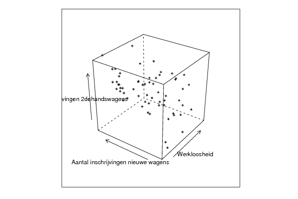
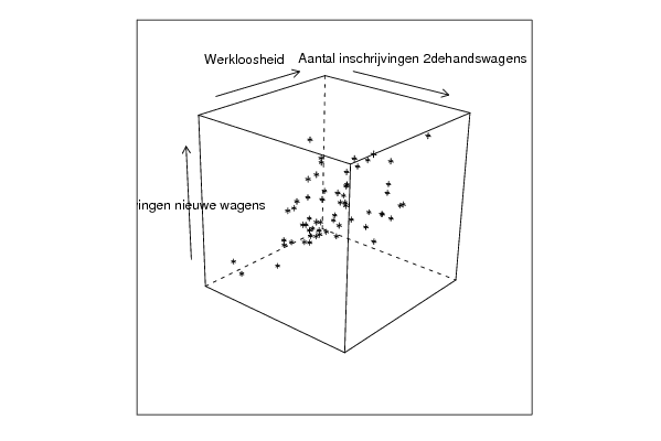
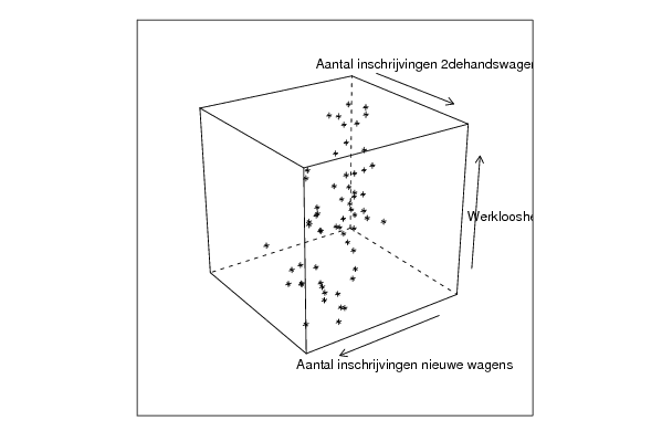
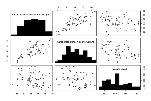
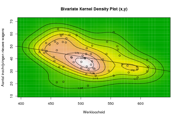
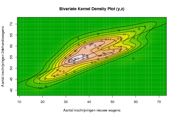
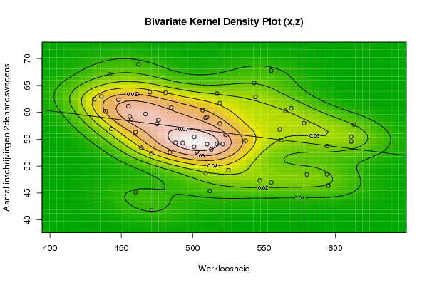
Trivariate Scatterplot Werkloosheid, aantal inschrijvingen nieuwe wagens en...

• QR Code (size=2)
• QR Code (size=3)
• QR Code (size=4)
• QR Code (size=5)
• QR Code (size=6)

493.000
481.000
462.000
457.000
442.000
439.000
488.000
521.000
501.000
485.000
464.000
460.000
467.000
460.000
448.000
443.000
436.000
431.000
484.000
510.000
513.000
503.000
471.000
471.000
476.000
475.000
470.000
461.000
455.000
456.000
517.000
525.000
523.000
519.000
509.000
512.000
519.000
517.000
510.000
509.000
501.000
507.000
569.000
580.000
578.000
565.000
547.000
555.000
562.000
561.000
555.000
544.000
537.000
543.000
594.000
611.000
613.000
611.000
594.000
595.000

58.972
59.249
63.955
53.785
52.760
44.795
37.348
32.370
32.717
40.974
33.591
21.124
58.608
46.865
51.378
46.235
47.206
45.382
41.227
33.795
31.295
42.625
33.625
21.538
56.421
53.152
53.536
52.408
41.454
38.271
35.306
26.414
31.917
38.030
27.534
18.387
50.556
43.901
48.572
43.899
37.532
40.357
35.489
29.027
34.485
42.598
30.306
26.451
47.460
50.104
61.465
53.726
39.477
43.895
31.481
29.896
33.842
39.120
33.702
25.094

54.281
63.654
68.918
58.686
67.074
60.183
54.326
54.085
53.564
60.873
53.398
45.164
59.672
56.298
62.361
56.930
62.954
62.431
52.528
54.060
53.093
52.695
52.333
41.747
58.576
57.851
63.721
63.384
61.141
59.231
63.472
49.214
55.816
61.713
48.664
45.351
57.888
54.091
59.098
58.962
55.433
60.403
60.721
48.440
57.981
60.258
47.312
46.980
54.846
56.824
67.744
62.849
54.691
65.461
53.724
54.560
57.722
55.458
48.490
46.362

x <- array(x,dim=c(length(x),1))
colnames(x) <- par5
y <- array(y,dim=c(length(y),1))
colnames(y) <- par6
z <- array(z,dim=c(length(z),1))
colnames(z) <- par7
d <- data.frame(cbind(z,y,x))
colnames(d) <- list(par7,par6,par5)
par1 <- as.numeric(par1)
par2 <- as.numeric(par2)
if (par1>500) par1 <- 500
if (par2>500) par2 <- 500
if (par1<10) par1 <- 10
if (par2<10) par2 <- 10
library(GenKern)
library(lattice)
panel.hist <- function(x, ...)
{
usr <- par('usr'); on.exit(par(usr))
par(usr = c(usr[1:2], 0, 1.5) )
h <- hist(x, plot = FALSE)
breaks <- h$breaks; nB <- length(breaks)
y <- h$counts; y <- y/max(y)
rect(breaks[-nB], 0, breaks[-1], y, col='black', ...)
}
bitmap(file='cloud1.png')
cloud(z~x*y, screen = list(x=-45, y=45, z=35),xlab=par5,ylab=par6,zlab=par7)
dev.off()
bitmap(file='cloud2.png')
cloud(z~x*y, screen = list(x=35, y=45, z=25),xlab=par5,ylab=par6,zlab=par7)
dev.off()
bitmap(file='cloud3.png')
cloud(z~x*y, screen = list(x=35, y=-25, z=90),xlab=par5,ylab=par6,zlab=par7)
dev.off()
bitmap(file='pairs.png')
pairs(d,diag.panel=panel.hist)
dev.off()
x <- as.vector(x)
y <- as.vector(y)
z <- as.vector(z)
bitmap(file='bidensity1.png')
op <- KernSur(x,y, xgridsize=par1, ygridsize=par2, correlation=cor(x,y), xbandwidth=dpik(x), ybandwidth=dpik(y))
image(op$xords, op$yords, op$zden, col=terrain.colors(100), axes=TRUE,main='Bivariate Kernel Density Plot (x,y)',xlab=par5,ylab=par6)
if (par3=='Y') contour(op$xords, op$yords, op$zden, add=TRUE)
if (par4=='Y') points(x,y)
(r<-lm(y ~ x))
abline(r)
box()
dev.off()
bitmap(file='bidensity2.png')
op <- KernSur(y,z, xgridsize=par1, ygridsize=par2, correlation=cor(y,z), xbandwidth=dpik(y), ybandwidth=dpik(z))
op
image(op$xords, op$yords, op$zden, col=terrain.colors(100), axes=TRUE,main='Bivariate Kernel Density Plot (y,z)',xlab=par6,ylab=par7)
if (par3=='Y') contour(op$xords, op$yords, op$zden, add=TRUE)
if (par4=='Y') points(y,z)
(r<-lm(z ~ y))
abline(r)
box()
dev.off()
bitmap(file='bidensity3.png')
op <- KernSur(x,z, xgridsize=par1, ygridsize=par2, correlation=cor(x,z), xbandwidth=dpik(x), ybandwidth=dpik(z))
op
image(op$xords, op$yords, op$zden, col=terrain.colors(100), axes=TRUE,main='Bivariate Kernel Density Plot (x,z)',xlab=par5,ylab=par7)
if (par3=='Y') contour(op$xords, op$yords, op$zden, add=TRUE)
if (par4=='Y') points(x,z)
(r<-lm(z ~ x))
abline(r)
box()
dev.off()