Free Statistics
of Irreproducible Research!
Description of Statistical Computation | |||||||||||||||||||||||||||||||||||||||||||||
|---|---|---|---|---|---|---|---|---|---|---|---|---|---|---|---|---|---|---|---|---|---|---|---|---|---|---|---|---|---|---|---|---|---|---|---|---|---|---|---|---|---|---|---|---|---|
| Author's title | |||||||||||||||||||||||||||||||||||||||||||||
| Author | *The author of this computation has been verified* | ||||||||||||||||||||||||||||||||||||||||||||
| R Software Module | rwasp_bidensity.wasp | ||||||||||||||||||||||||||||||||||||||||||||
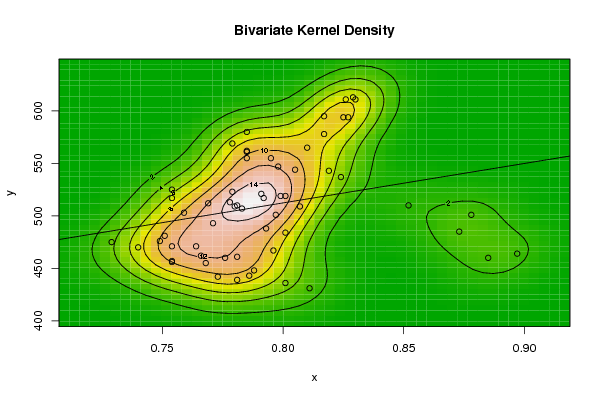
| Title produced by software | Bivariate Kernel Density Estimation | ||||||||||||||||||||||||||||||||||||||||||||
| Date of computation | Mon, 10 Nov 2008 09:58:43 -0700 | ||||||||||||||||||||||||||||||||||||||||||||
| Cite this page as follows | Statistical Computations at FreeStatistics.org, Office for Research Development and Education, URL https://freestatistics.org/blog/index.php?v=date/2008/Nov/10/t1226336368gvwpkmwiudkj9jt.htm/, Retrieved Sun, 19 May 2024 12:14:57 +0000 | ||||||||||||||||||||||||||||||||||||||||||||
| Statistical Computations at FreeStatistics.org, Office for Research Development and Education, URL https://freestatistics.org/blog/index.php?pk=23139, Retrieved Sun, 19 May 2024 12:14:57 +0000 | |||||||||||||||||||||||||||||||||||||||||||||
| QR Codes: | |||||||||||||||||||||||||||||||||||||||||||||
|
| |||||||||||||||||||||||||||||||||||||||||||||
| Original text written by user: | |||||||||||||||||||||||||||||||||||||||||||||
| IsPrivate? | No (this computation is public) | ||||||||||||||||||||||||||||||||||||||||||||
| User-defined keywords | |||||||||||||||||||||||||||||||||||||||||||||
| Estimated Impact | 185 | ||||||||||||||||||||||||||||||||||||||||||||
Tree of Dependent Computations | |||||||||||||||||||||||||||||||||||||||||||||
| Family? (F = Feedback message, R = changed R code, M = changed R Module, P = changed Parameters, D = changed Data) | |||||||||||||||||||||||||||||||||||||||||||||
| F [Bivariate Kernel Density Estimation] [Bivariate Kernel ...] [2008-11-10 16:53:50] [819b576fab25b35cfda70f80599828ec] F D [Bivariate Kernel Density Estimation] [Bivaritae Kernel ...] [2008-11-10 16:58:43] [e08fee3874f3333d6b7a377a061b860d] [Current] F D [Bivariate Kernel Density Estimation] [Bivariate Kernel ...] [2008-11-10 17:00:38] [819b576fab25b35cfda70f80599828ec] - D [Bivariate Kernel Density Estimation] [paper 1.9 bivaria...] [2008-12-05 19:08:16] [819b576fab25b35cfda70f80599828ec] F RMPD [Partial Correlation] [Partial Correlati...] [2008-11-10 17:08:28] [819b576fab25b35cfda70f80599828ec] - D [Partial Correlation] [Partial Correlati...] [2008-11-10 17:13:48] [819b576fab25b35cfda70f80599828ec] F D [Partial Correlation] [Partial Correlati...] [2008-11-10 17:17:49] [819b576fab25b35cfda70f80599828ec] - RMPD [Trivariate Scatterplots] [Trivariate Scatte...] [2008-11-10 17:21:24] [819b576fab25b35cfda70f80599828ec] - P [Trivariate Scatterplots] [Trivariate Scatte...] [2008-11-10 17:31:18] [819b576fab25b35cfda70f80599828ec] F RMPD [Hierarchical Clustering] [Hierarchical Clus...] [2008-11-10 17:36:33] [819b576fab25b35cfda70f80599828ec] F RM D [Box-Cox Linearity Plot] [Box-Cox linearity...] [2008-11-11 14:51:35] [6fea0e9a9b3b29a63badf2c274e82506] - RMPD [Box-Cox Normality Plot] [Box-Cox Normality...] [2008-11-10 17:45:50] [819b576fab25b35cfda70f80599828ec] F D [Box-Cox Normality Plot] [Box Cox normality...] [2008-11-11 15:12:02] [6fea0e9a9b3b29a63badf2c274e82506] - RMPD [Maximum-likelihood Fitting - Normal Distribution] [Maximum-likelihoo...] [2008-11-10 17:50:35] [819b576fab25b35cfda70f80599828ec] F PD [Maximum-likelihood Fitting - Normal Distribution] [Maximum-likelihoo...] [2008-11-11 15:33:55] [819b576fab25b35cfda70f80599828ec] - RMPD [Trivariate Scatterplots] [Trivariate Scatte...] [2008-11-10 17:27:05] [819b576fab25b35cfda70f80599828ec] | |||||||||||||||||||||||||||||||||||||||||||||
| Feedback Forum | |||||||||||||||||||||||||||||||||||||||||||||
Post a new message | |||||||||||||||||||||||||||||||||||||||||||||
Dataset | |||||||||||||||||||||||||||||||||||||||||||||
| Dataseries X: | |||||||||||||||||||||||||||||||||||||||||||||
0.771 0.751 0.766 0.754 0.773 0.781 0.793 0.791 0.878 0.873 0.897 0.885 0.796 0.776 0.788 0.786 0.801 0.811 0.801 0.781 0.778 0.759 0.764 0.754 0.749 0.729 0.740 0.781 0.768 0.754 0.754 0.754 0.779 0.799 0.780 0.769 0.801 0.792 0.852 0.807 0.797 0.783 0.779 0.785 0.817 0.810 0.798 0.795 0.785 0.785 0.785 0.805 0.824 0.819 0.827 0.826 0.829 0.830 0.825 0.817 | |||||||||||||||||||||||||||||||||||||||||||||
| Dataseries Y: | |||||||||||||||||||||||||||||||||||||||||||||
493.000 481.000 462.000 457.000 442.000 439.000 488.000 521.000 501.000 485.000 464.000 460.000 467.000 460.000 448.000 443.000 436.000 431.000 484.000 510.000 513.000 503.000 471.000 471.000 476.000 475.000 470.000 461.000 455.000 456.000 517.000 525.000 523.000 519.000 509.000 512.000 519.000 517.000 510.000 509.000 501.000 507.000 569.000 580.000 578.000 565.000 547.000 555.000 562.000 561.000 555.000 544.000 537.000 543.000 594.000 611.000 613.000 611.000 594.000 595.000 | |||||||||||||||||||||||||||||||||||||||||||||
Tables (Output of Computation) | |||||||||||||||||||||||||||||||||||||||||||||
| |||||||||||||||||||||||||||||||||||||||||||||
Figures (Output of Computation) | |||||||||||||||||||||||||||||||||||||||||||||
Input Parameters & R Code | |||||||||||||||||||||||||||||||||||||||||||||
| Parameters (Session): | |||||||||||||||||||||||||||||||||||||||||||||
| par1 = 50 ; par2 = 50 ; par3 = 0 ; par4 = 0 ; par5 = 0 ; par6 = Y ; par7 = Y ; | |||||||||||||||||||||||||||||||||||||||||||||
| Parameters (R input): | |||||||||||||||||||||||||||||||||||||||||||||
| par1 = 50 ; par2 = 50 ; par3 = 0 ; par4 = 0 ; par5 = 0 ; par6 = Y ; par7 = Y ; | |||||||||||||||||||||||||||||||||||||||||||||
| R code (references can be found in the software module): | |||||||||||||||||||||||||||||||||||||||||||||
par1 <- as(par1,'numeric') | |||||||||||||||||||||||||||||||||||||||||||||