Free Statistics
of Irreproducible Research!
Description of Statistical Computation | |||||||||||||||||||||||||||||||||||||||||||||
|---|---|---|---|---|---|---|---|---|---|---|---|---|---|---|---|---|---|---|---|---|---|---|---|---|---|---|---|---|---|---|---|---|---|---|---|---|---|---|---|---|---|---|---|---|---|
| Author's title | |||||||||||||||||||||||||||||||||||||||||||||
| Author | *Unverified author* | ||||||||||||||||||||||||||||||||||||||||||||
| R Software Module | rwasp_boxcoxlin.wasp | ||||||||||||||||||||||||||||||||||||||||||||
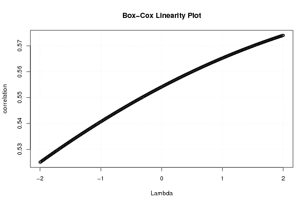
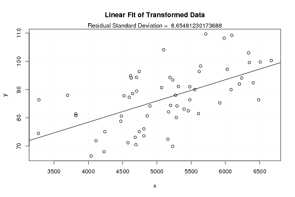
| Title produced by software | Box-Cox Linearity Plot | ||||||||||||||||||||||||||||||||||||||||||||
| Date of computation | Mon, 10 Nov 2008 07:07:00 -0700 | ||||||||||||||||||||||||||||||||||||||||||||
| Cite this page as follows | Statistical Computations at FreeStatistics.org, Office for Research Development and Education, URL https://freestatistics.org/blog/index.php?v=date/2008/Nov/10/t1226326085ag4uftj36ih9jvr.htm/, Retrieved Sun, 19 May 2024 11:11:38 +0000 | ||||||||||||||||||||||||||||||||||||||||||||
| Statistical Computations at FreeStatistics.org, Office for Research Development and Education, URL https://freestatistics.org/blog/index.php?pk=23065, Retrieved Sun, 19 May 2024 11:11:38 +0000 | |||||||||||||||||||||||||||||||||||||||||||||
| QR Codes: | |||||||||||||||||||||||||||||||||||||||||||||
|
| |||||||||||||||||||||||||||||||||||||||||||||
| Original text written by user: | |||||||||||||||||||||||||||||||||||||||||||||
| IsPrivate? | No (this computation is public) | ||||||||||||||||||||||||||||||||||||||||||||
| User-defined keywords | box cox linearity plot Q2 | ||||||||||||||||||||||||||||||||||||||||||||
| Estimated Impact | 229 | ||||||||||||||||||||||||||||||||||||||||||||
Tree of Dependent Computations | |||||||||||||||||||||||||||||||||||||||||||||
| Family? (F = Feedback message, R = changed R code, M = changed R Module, P = changed Parameters, D = changed Data) | |||||||||||||||||||||||||||||||||||||||||||||
| - [Box-Cox Linearity Plot] [] [2007-10-30 20:15:08] [d63889a2cb43a84e31f95f02a72561da] F R D [Box-Cox Linearity Plot] [box cox linearity...] [2008-11-10 14:07:00] [d8c5724db236abb5950452133b88474d] [Current] | |||||||||||||||||||||||||||||||||||||||||||||
| Feedback Forum | |||||||||||||||||||||||||||||||||||||||||||||
Post a new message | |||||||||||||||||||||||||||||||||||||||||||||
Dataset | |||||||||||||||||||||||||||||||||||||||||||||
| Dataseries X: | |||||||||||||||||||||||||||||||||||||||||||||
110,40 96,40 101,90 106,20 81,00 94,70 101,00 109,40 102,30 90,70 96,20 96,10 106,00 103,10 102,00 104,70 86,00 92,10 106,90 112,60 101,70 92,00 97,40 97,00 105,40 102,70 98,10 104,50 87,40 89,90 109,80 111,70 98,60 96,90 95,10 97,00 112,70 102,90 97,40 111,40 87,40 96,80 114,10 110,30 103,90 101,60 94,60 95,90 104,70 102,80 98,10 113,90 80,90 95,70 113,20 105,90 108,80 102,30 99,00 100,70 115,50 | |||||||||||||||||||||||||||||||||||||||||||||
| Dataseries Y: | |||||||||||||||||||||||||||||||||||||||||||||
109,20 88,60 94,30 98,30 86,40 80,60 104,10 108,20 93,40 71,90 94,10 94,90 96,40 91,10 84,40 86,40 88,00 75,10 109,70 103,00 82,10 68,00 96,40 94,30 90,00 88,00 76,10 82,50 81,40 66,50 97,20 94,10 80,70 70,50 87,80 89,50 99,60 84,20 75,10 92,00 80,80 73,10 99,80 90,00 83,10 72,40 78,80 87,30 91,00 80,10 73,60 86,40 74,50 71,20 92,40 81,50 85,30 69,90 84,20 90,70 100,30 | |||||||||||||||||||||||||||||||||||||||||||||
Tables (Output of Computation) | |||||||||||||||||||||||||||||||||||||||||||||
| |||||||||||||||||||||||||||||||||||||||||||||
Figures (Output of Computation) | |||||||||||||||||||||||||||||||||||||||||||||
Input Parameters & R Code | |||||||||||||||||||||||||||||||||||||||||||||
| Parameters (Session): | |||||||||||||||||||||||||||||||||||||||||||||
| Parameters (R input): | |||||||||||||||||||||||||||||||||||||||||||||
| R code (references can be found in the software module): | |||||||||||||||||||||||||||||||||||||||||||||
n <- length(x) | |||||||||||||||||||||||||||||||||||||||||||||