Free Statistics
of Irreproducible Research!
Description of Statistical Computation | |||||||||||||||||||||||||||||||||||||
|---|---|---|---|---|---|---|---|---|---|---|---|---|---|---|---|---|---|---|---|---|---|---|---|---|---|---|---|---|---|---|---|---|---|---|---|---|---|
| Author's title | |||||||||||||||||||||||||||||||||||||
| Author | *The author of this computation has been verified* | ||||||||||||||||||||||||||||||||||||
| R Software Module | rwasp_boxcoxnorm.wasp | ||||||||||||||||||||||||||||||||||||
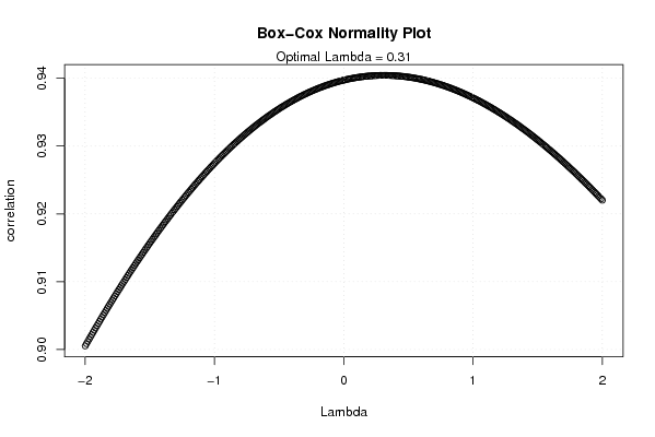
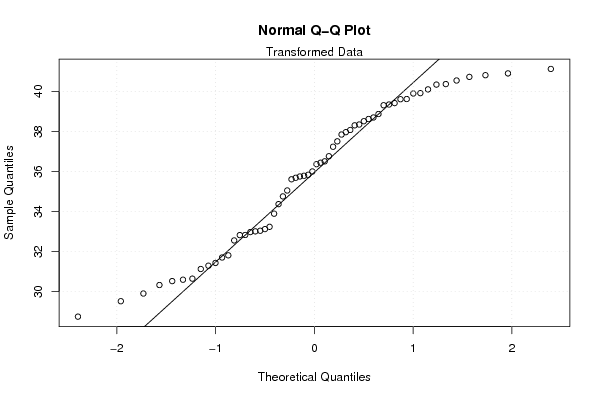
| Title produced by software | Box-Cox Normality Plot | ||||||||||||||||||||||||||||||||||||
| Date of computation | Mon, 10 Nov 2008 04:55:49 -0700 | ||||||||||||||||||||||||||||||||||||
| Cite this page as follows | Statistical Computations at FreeStatistics.org, Office for Research Development and Education, URL https://freestatistics.org/blog/index.php?v=date/2008/Nov/10/t1226318233f53llulqcijib33.htm/, Retrieved Sun, 19 May 2024 10:46:49 +0000 | ||||||||||||||||||||||||||||||||||||
| Statistical Computations at FreeStatistics.org, Office for Research Development and Education, URL https://freestatistics.org/blog/index.php?pk=22970, Retrieved Sun, 19 May 2024 10:46:49 +0000 | |||||||||||||||||||||||||||||||||||||
| QR Codes: | |||||||||||||||||||||||||||||||||||||
|
| |||||||||||||||||||||||||||||||||||||
| Original text written by user: | |||||||||||||||||||||||||||||||||||||
| IsPrivate? | No (this computation is public) | ||||||||||||||||||||||||||||||||||||
| User-defined keywords | |||||||||||||||||||||||||||||||||||||
| Estimated Impact | 239 | ||||||||||||||||||||||||||||||||||||
Tree of Dependent Computations | |||||||||||||||||||||||||||||||||||||
| Family? (F = Feedback message, R = changed R code, M = changed R Module, P = changed Parameters, D = changed Data) | |||||||||||||||||||||||||||||||||||||
| F [Bivariate Kernel Density Estimation] [Various EDA topic...] [2008-11-07 10:38:01] [e5d91604aae608e98a8ea24759233f66] F RMPD [Trivariate Scatterplots] [Various EDA topic...] [2008-11-07 10:42:57] [e5d91604aae608e98a8ea24759233f66] F RMPD [Box-Cox Linearity Plot] [Various EDA topic...] [2008-11-07 11:06:19] [e5d91604aae608e98a8ea24759233f66] F RM D [Box-Cox Normality Plot] [Various EDA topic...] [2008-11-10 11:55:49] [55ca0ca4a201c9689dcf5fae352c92eb] [Current] F RMPD [Maximum-likelihood Fitting - Normal Distribution] [Various EDA topic...] [2008-11-10 12:02:10] [e5d91604aae608e98a8ea24759233f66] - RMPD [Testing Variance - Critical Value (Region)] [Various types of ...] [2008-11-10 12:36:06] [e5d91604aae608e98a8ea24759233f66] - P [Testing Variance - Critical Value (Region)] [Various types of ...] [2008-11-10 12:44:47] [e5d91604aae608e98a8ea24759233f66] - RMPD [Notched Boxplots] [Various types of ...] [2008-11-10 13:05:18] [e5d91604aae608e98a8ea24759233f66] - RMPD [Testing Variance - p-value (probability)] [Various types of ...] [2008-11-10 12:39:28] [e5d91604aae608e98a8ea24759233f66] | |||||||||||||||||||||||||||||||||||||
| Feedback Forum | |||||||||||||||||||||||||||||||||||||
Post a new message | |||||||||||||||||||||||||||||||||||||
Dataset | |||||||||||||||||||||||||||||||||||||
| Dataseries X: | |||||||||||||||||||||||||||||||||||||
1946,81 1765,9 1635,25 1833,42 1910,43 1959,67 1969,6 2061,41 2093,48 2120,88 2174,56 2196,72 2350,44 2440,25 2408,64 2472,81 2407,6 2454,62 2448,05 2497,84 2645,64 2756,76 2849,27 2921,44 3080,58 3106,22 3119,31 3061,26 3097,31 3161,69 3257,16 3277,01 3295,32 3363,99 3494,17 3667,03 3813,06 3917,96 3895,51 3733,22 3801,06 3570,12 3701,61 3862,27 3970,1 4138,52 4199,75 4290,89 4443,91 4502,64 4356,98 4591,27 4696,96 4621,4 4562,84 4202,52 4296,49 4435,23 4105,18 4116,68 | |||||||||||||||||||||||||||||||||||||
Tables (Output of Computation) | |||||||||||||||||||||||||||||||||||||
| |||||||||||||||||||||||||||||||||||||
Figures (Output of Computation) | |||||||||||||||||||||||||||||||||||||
Input Parameters & R Code | |||||||||||||||||||||||||||||||||||||
| Parameters (Session): | |||||||||||||||||||||||||||||||||||||
| Parameters (R input): | |||||||||||||||||||||||||||||||||||||
| R code (references can be found in the software module): | |||||||||||||||||||||||||||||||||||||
n <- length(x) | |||||||||||||||||||||||||||||||||||||