Repository of Reproducible Computations

Free Statistics

of Irreproducible Research!

Author's title

Author

*The author of this computation has been verified*

R Software Module

rwasp_bidensity.wasp

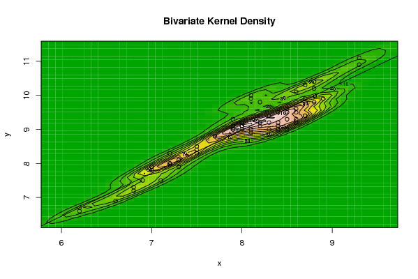
Title produced by software

Bivariate Kernel Density Estimation

Date of computation

Mon, 10 Nov 2008 04:26:35 -0700

Cite this page as follows

Statistical Computations at FreeStatistics.org, Office for Research Development and Education, URL https://freestatistics.org/blog/index.php?v=date/2008/Nov/10/t12263164813bgv4nf4s4qyulw.htm/, Retrieved Sun, 19 May 2024 12:38:18 +0000

Statistical Computations at FreeStatistics.org, Office for Research Development and Education, URL https://freestatistics.org/blog/index.php?pk=22953, Retrieved Sun, 19 May 2024 12:38:18 +0000

QR Codes:

Paste this QR Code to cite your computation.

Original text written by user:

IsPrivate?

No (this computation is public)

User-defined keywords

Bivariate Kernel Density Estimation

Estimated Impact

193

Family? (F = Feedback message, R = changed R code, M = changed R Module, P = changed Parameters, D = changed Data)

-     [Univariate Data Series] [Totaal % werkzoek...] [2008-10-13 17:09:30] [b635de6fc42b001d22cbe6e730fec936]
F RMP   [Central Tendency] [Totaal % werkzoek...] [2008-10-20 17:37:42] [b635de6fc42b001d22cbe6e730fec936]
- RMPD    [Histogram] [Histogram percent...] [2008-10-21 07:16:54] [b635de6fc42b001d22cbe6e730fec936]
- RMPD      [Back to Back Histogram] [Back to back kolo...] [2008-10-21 07:29:52] [b635de6fc42b001d22cbe6e730fec936]
-    D        [Back to Back Histogram] [Back to back hist...] [2008-10-24 10:56:18] [b635de6fc42b001d22cbe6e730fec936]
F RMP             [Bivariate Kernel Density Estimation] [Bivariate Kernel ...] [2008-11-10 11:26:35] [f4b2017b314c03698059f43b95818e67] [Current]

Feedback Forum

2008-11-10 11:46:47 [Bas van Keken] [reply] 
X as = Totaal % werkzoekenden 
Y as = Totaal % werkzoekende vrouwen
2008-11-12 18:04:17 [Romina Machiels] [reply] 
In Q1 werden de juiste berekeningen gemaakt, er werd enkel onvoldoende uitleg gegeven. Bij de bivariate density zie je dat er tussen de tijdreeksen een hoge correlatie is. 
Bij de partial correlation word bv bij de correlatie van x met y, de invloed van z weggezuiverd. De correlatie van 2 kan een heel vertekend beeld geven omdat ze onder invloed staan van een derde, bij de partial correlation word deze invloed echter weggezuiverd zodat we een juist beeld krijgen van de correlatie van x en y.

Post a new message

Dataseries X:

Download CSV

Histogram

Boxplots

8.4
8.4
8.4
8.6
8.9
8.8
8.3
7.5
7.2
7.5
8.8
9.3
9.3
8.7
8.2
8.3
8.5
8.6
8.6
8.2
8.1
8
8.6
8.7
8.8
8.5
8.4
8.5
8.7
8.7
8.6
8.5
8.3
8.1
8.2
8.1
8.1
7.9
7.9
7.9
8
8
7.9
8
7.7
7.2
7.5
7.3
7
7
7
7.2
7.3
7.1
6.8
6.6
6.2
6.2
6.8
6.9

Dataseries Y:

Download CSV

Histogram

9.5
9.1
9
9.3
9.9
9.8
9.4
8.3
8
8.5
10.4
11.1
10.9
9.9
9.2
9.2
9.5
9.6
9.5
9.1
8.9
9
10.1
10.3
10.2
9.6
9.2
9.3
9.4
9.4
9.2
9
9
9
9.8
10
9.9
9.3
9
9
9.1
9.1
9.1
9.2
8.8
8.3
8.4
8.1
7.8
7.9
7.9
8
7.9
7.5
7.2
6.9
6.6
6.7
7.3
7.5

Summary of computational transaction
Raw Input	view raw input (R code)
Raw Output	view raw output of R engine
Computing time	3 seconds
R Server	'Herman Ole Andreas Wold' @ 193.190.124.10:1001

\begin{tabular}{lllllllll}
\hline
Summary of computational transaction \tabularnewline
Raw Input & view raw input (R code)  \tabularnewline
Raw Output & view raw output of R engine  \tabularnewline
Computing time & 3 seconds \tabularnewline
R Server & 'Herman Ole Andreas Wold' @ 193.190.124.10:1001 \tabularnewline
\hline
\end{tabular}
%Source: https://freestatistics.org/blog/index.php?pk=22953&T=0

[TABLE]
[ROW][C]Summary of computational transaction[/C][/ROW]
[ROW][C]Raw Input[/C][C]view raw input (R code) [/C][/ROW]
[ROW][C]Raw Output[/C][C]view raw output of R engine [/C][/ROW]
[ROW][C]Computing time[/C][C]3 seconds[/C][/ROW]
[ROW][C]R Server[/C][C]'Herman Ole Andreas Wold' @ 193.190.124.10:1001[/C][/ROW]
[/TABLE]
Source: https://freestatistics.org/blog/index.php?pk=22953&T=0

Globally Unique Identifier (entire table): ba.freestatistics.org/blog/index.php?pk=22953&T=0

As an alternative you can also use a QR Code:

The GUIDs for individual cells are displayed in the table below:

Summary of computational transaction
Raw Input	view raw input (R code)
Raw Output	view raw output of R engine
Computing time	3 seconds
R Server	'Herman Ole Andreas Wold' @ 193.190.124.10:1001

Bandwidth
x axis	0.256788257826575
y axis	0.28933865608174
Correlation
correlation used in KDE	0.947355649706108
correlation(x,y)	0.947355649706108

\begin{tabular}{lllllllll}
\hline
Bandwidth \tabularnewline
x axis & 0.256788257826575 \tabularnewline
y axis & 0.28933865608174 \tabularnewline
Correlation \tabularnewline
correlation used in KDE & 0.947355649706108 \tabularnewline
correlation(x,y) & 0.947355649706108 \tabularnewline
\hline
\end{tabular}
%Source: https://freestatistics.org/blog/index.php?pk=22953&T=1

[TABLE]
[ROW][C]Bandwidth[/C][/ROW]
[ROW][C]x axis[/C][C]0.256788257826575[/C][/ROW]
[ROW][C]y axis[/C][C]0.28933865608174[/C][/ROW]
[ROW][C]Correlation[/C][/ROW]
[ROW][C]correlation used in KDE[/C][C]0.947355649706108[/C][/ROW]
[ROW][C]correlation(x,y)[/C][C]0.947355649706108[/C][/ROW]
[/TABLE]
Source: https://freestatistics.org/blog/index.php?pk=22953&T=1

Globally Unique Identifier (entire table): ba.freestatistics.org/blog/index.php?pk=22953&T=1

As an alternative you can also use a QR Code:

The GUIDs for individual cells are displayed in the table below:

Bandwidth
x axis	0.256788257826575
y axis	0.28933865608174
Correlation
correlation used in KDE	0.947355649706108
correlation(x,y)	0.947355649706108

Figure 1

PNG link

Postscript link

PDF link

Parameters (Session):

par1 = 50 ; par2 = 50 ; par3 = 0 ; par4 = 0 ; par5 = 0 ; par6 = Y ; par7 = Y ;

Parameters (R input):

par1 = 50 ; par2 = 50 ; par3 = 0 ; par4 = 0 ; par5 = 0 ; par6 = Y ; par7 = Y ;

R code (references can be found in the software module):

par1 <- as(par1,'numeric')
par2 <- as(par2,'numeric')
par3 <- as(par3,'numeric')
par4 <- as(par4,'numeric')
par5 <- as(par5,'numeric')
library('GenKern')
if (par3==0) par3 <- dpik(x)
if (par4==0) par4 <- dpik(y)
if (par5==0) par5 <- cor(x,y)
if (par1 > 500) par1 <- 500
if (par2 > 500) par2 <- 500
bitmap(file='bidensity.png')
op <- KernSur(x,y, xgridsize=par1, ygridsize=par2, correlation=par5, xbandwidth=par3, ybandwidth=par4)
image(op$xords, op$yords, op$zden, col=terrain.colors(100), axes=TRUE,main=main,xlab=xlab,ylab=ylab)
if (par6=='Y') contour(op$xords, op$yords, op$zden, add=TRUE)
if (par7=='Y') points(x,y)
(r<-lm(y ~ x))
abline(r)
box()
dev.off()
load(file='createtable')
a<-table.start()
a<-table.row.start(a)
a<-table.element(a,'Bandwidth',2,TRUE)
a<-table.row.end(a)
a<-table.row.start(a)
a<-table.element(a,'x axis',header=TRUE)
a<-table.element(a,par3)
a<-table.row.end(a)
a<-table.row.start(a)
a<-table.element(a,'y axis',header=TRUE)
a<-table.element(a,par4)
a<-table.row.end(a)
a<-table.row.start(a)
a<-table.element(a,'Correlation',2,TRUE)
a<-table.row.end(a)
a<-table.row.start(a)
a<-table.element(a,'correlation used in KDE',header=TRUE)
a<-table.element(a,par5)
a<-table.row.end(a)
a<-table.row.start(a)
a<-table.element(a,'correlation(x,y)',header=TRUE)
a<-table.element(a,cor(x,y))
a<-table.row.end(a)
a<-table.end(a)
table.save(a,file='mytable.tab')

Free Statistics

Description of Statistical Computation

Tree of Dependent Computations

Dataset

Tables (Output of Computation)

Figures (Output of Computation)

Input Parameters & R Code