Free Statistics
of Irreproducible Research!
Description of Statistical Computation | |||||||||||||||||||||||||||||||||||||
|---|---|---|---|---|---|---|---|---|---|---|---|---|---|---|---|---|---|---|---|---|---|---|---|---|---|---|---|---|---|---|---|---|---|---|---|---|---|
| Author's title | |||||||||||||||||||||||||||||||||||||
| Author | *The author of this computation has been verified* | ||||||||||||||||||||||||||||||||||||
| R Software Module | rwasp_boxcoxnorm.wasp | ||||||||||||||||||||||||||||||||||||
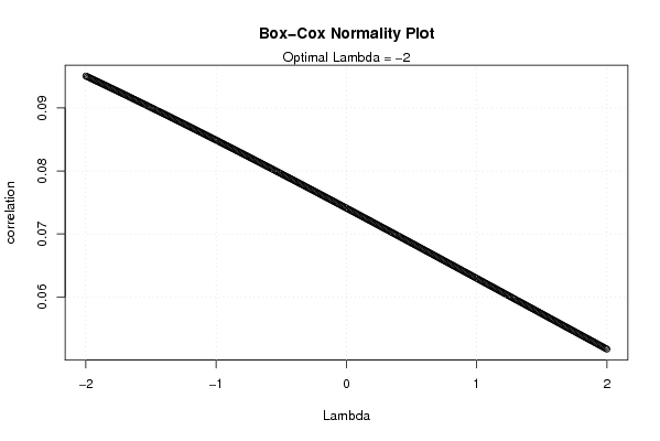
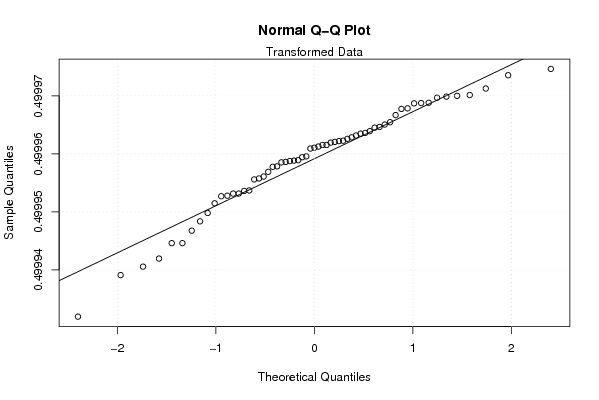
| Title produced by software | Box-Cox Normality Plot | ||||||||||||||||||||||||||||||||||||
| Date of computation | Sun, 09 Nov 2008 05:35:32 -0700 | ||||||||||||||||||||||||||||||||||||
| Cite this page as follows | Statistical Computations at FreeStatistics.org, Office for Research Development and Education, URL https://freestatistics.org/blog/index.php?v=date/2008/Nov/09/t1226234197hponog5sedwvtby.htm/, Retrieved Sun, 13 Jul 2025 09:40:28 +0000 | ||||||||||||||||||||||||||||||||||||
| Statistical Computations at FreeStatistics.org, Office for Research Development and Education, URL https://freestatistics.org/blog/index.php?pk=22725, Retrieved Sun, 13 Jul 2025 09:40:28 +0000 | |||||||||||||||||||||||||||||||||||||
| QR Codes: | |||||||||||||||||||||||||||||||||||||
|
| |||||||||||||||||||||||||||||||||||||
| Original text written by user: | |||||||||||||||||||||||||||||||||||||
| IsPrivate? | No (this computation is public) | ||||||||||||||||||||||||||||||||||||
| User-defined keywords | |||||||||||||||||||||||||||||||||||||
| Estimated Impact | 282 | ||||||||||||||||||||||||||||||||||||
Tree of Dependent Computations | |||||||||||||||||||||||||||||||||||||
| Family? (F = Feedback message, R = changed R code, M = changed R Module, P = changed Parameters, D = changed Data) | |||||||||||||||||||||||||||||||||||||
| F [Partial Correlation] [Partial correlation] [2008-11-08 12:17:14] [82d201ca7b4e7cd2c6f885d29b5b6937] F RM D [Box-Cox Normality Plot] [Box Cox Normality] [2008-11-09 12:35:32] [00a0a665d7a07edd2e460056b0c0c354] [Current] F [Box-Cox Normality Plot] [Box cox normality] [2008-11-10 22:32:57] [8d78428855b119373cac369316c08983] | |||||||||||||||||||||||||||||||||||||
| Feedback Forum | |||||||||||||||||||||||||||||||||||||
Post a new message | |||||||||||||||||||||||||||||||||||||
Dataset | |||||||||||||||||||||||||||||||||||||
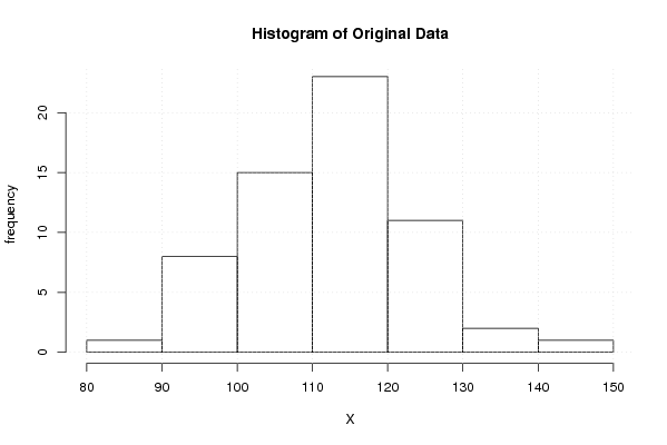
| Dataseries X: | |||||||||||||||||||||||||||||||||||||
118,9 108,8 115,6 95,0 92,8 108,9 109,8 106,1 102,8 98,4 85,7 114,6 129,4 117,7 126,6 103,8 101,5 118,7 119,6 114,8 109,9 106,3 95,0 124,5 140,4 128,8 137,5 113,3 110,3 129,1 128,4 120,3 113,6 96,9 124,7 126,4 131,9 122,5 113,1 99,8 116,0 115,0 114,0 111,0 91,7 90,6 103,3 106,7 111,2 102,9 126,5 115,1 110,2 110,1 103,3 107,7 103,9 114,0 117,2 117,0 116,5 | |||||||||||||||||||||||||||||||||||||
Tables (Output of Computation) | |||||||||||||||||||||||||||||||||||||
| |||||||||||||||||||||||||||||||||||||
Figures (Output of Computation) | |||||||||||||||||||||||||||||||||||||
Input Parameters & R Code | |||||||||||||||||||||||||||||||||||||
| Parameters (Session): | |||||||||||||||||||||||||||||||||||||
| Parameters (R input): | |||||||||||||||||||||||||||||||||||||
| R code (references can be found in the software module): | |||||||||||||||||||||||||||||||||||||
n <- length(x) | |||||||||||||||||||||||||||||||||||||