Free Statistics
of Irreproducible Research!
Description of Statistical Computation | |||||||||||||||||||||
|---|---|---|---|---|---|---|---|---|---|---|---|---|---|---|---|---|---|---|---|---|---|
| Author's title | |||||||||||||||||||||
| Author | *The author of this computation has been verified* | ||||||||||||||||||||
| R Software Module | rwasp_cloud.wasp | ||||||||||||||||||||
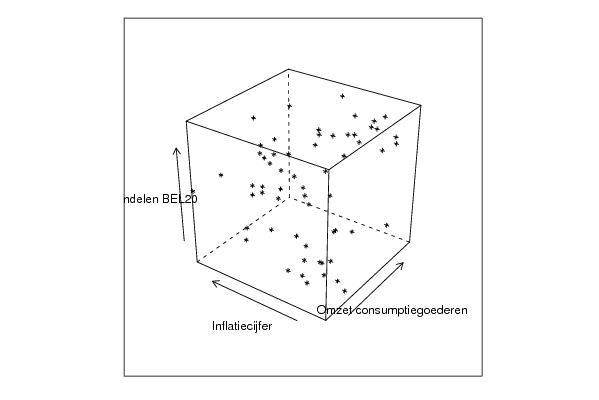
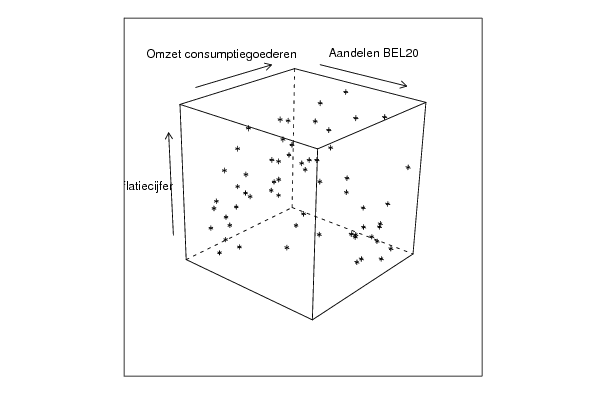
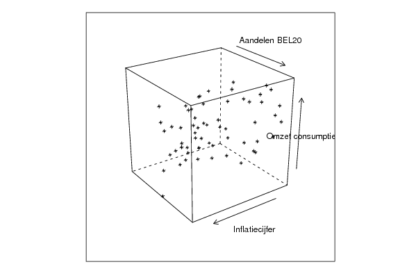
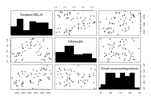
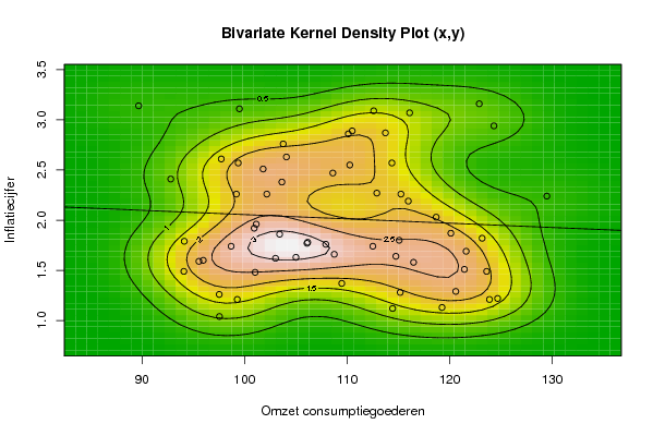
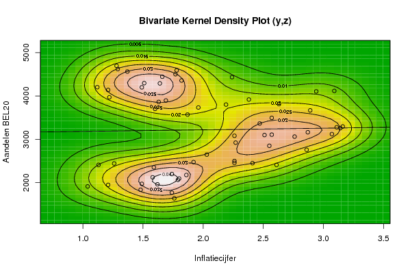
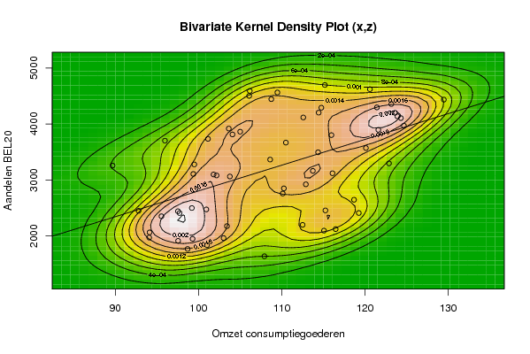
| Title produced by software | Trivariate Scatterplots | ||||||||||||||||||||
| Date of computation | Fri, 07 Nov 2008 03:42:57 -0700 | ||||||||||||||||||||
| Cite this page as follows | Statistical Computations at FreeStatistics.org, Office for Research Development and Education, URL https://freestatistics.org/blog/index.php?v=date/2008/Nov/07/t1226054703t35dip3qcg0cxcu.htm/, Retrieved Sun, 19 May 2024 05:57:42 +0000 | ||||||||||||||||||||
| Statistical Computations at FreeStatistics.org, Office for Research Development and Education, URL https://freestatistics.org/blog/index.php?pk=22468, Retrieved Sun, 19 May 2024 05:57:42 +0000 | |||||||||||||||||||||
| QR Codes: | |||||||||||||||||||||
|
| |||||||||||||||||||||
| Original text written by user: | |||||||||||||||||||||
| IsPrivate? | No (this computation is public) | ||||||||||||||||||||
| User-defined keywords | |||||||||||||||||||||
| Estimated Impact | 288 | ||||||||||||||||||||
Tree of Dependent Computations | |||||||||||||||||||||
| Family? (F = Feedback message, R = changed R code, M = changed R Module, P = changed Parameters, D = changed Data) | |||||||||||||||||||||
| F [Bivariate Kernel Density Estimation] [Various EDA topic...] [2008-11-07 10:38:01] [e5d91604aae608e98a8ea24759233f66] F RMPD [Trivariate Scatterplots] [Various EDA topic...] [2008-11-07 10:42:57] [55ca0ca4a201c9689dcf5fae352c92eb] [Current] F RMPD [Partial Correlation] [Various EDA topic...] [2008-11-07 10:48:55] [e5d91604aae608e98a8ea24759233f66] F RMPD [Box-Cox Linearity Plot] [Various EDA topic...] [2008-11-07 11:06:19] [e5d91604aae608e98a8ea24759233f66] F RM D [Box-Cox Normality Plot] [Various EDA topic...] [2008-11-10 11:55:49] [e5d91604aae608e98a8ea24759233f66] F RMPD [Maximum-likelihood Fitting - Normal Distribution] [Various EDA topic...] [2008-11-10 12:02:10] [e5d91604aae608e98a8ea24759233f66] - RMPD [Testing Variance - Critical Value (Region)] [Various types of ...] [2008-11-10 12:36:06] [e5d91604aae608e98a8ea24759233f66] - P [Testing Variance - Critical Value (Region)] [Various types of ...] [2008-11-10 12:44:47] [e5d91604aae608e98a8ea24759233f66] - RMPD [Notched Boxplots] [Various types of ...] [2008-11-10 13:05:18] [e5d91604aae608e98a8ea24759233f66] - RMPD [Testing Variance - p-value (probability)] [Various types of ...] [2008-11-10 12:39:28] [e5d91604aae608e98a8ea24759233f66] - RMPD [Kendall tau Correlation Matrix] [Various EDA topic...] [2008-11-07 11:03:18] [e5d91604aae608e98a8ea24759233f66] F RMPD [Testing Mean with known Variance - Critical Value] [Case - Q1] [2008-11-07 11:22:19] [e5d91604aae608e98a8ea24759233f66] F RM [Testing Mean with known Variance - p-value] [Case - Q2] [2008-11-07 11:40:30] [e5d91604aae608e98a8ea24759233f66] F RM [Testing Mean with known Variance - Type II Error] [Case - Q3] [2008-11-07 11:49:06] [e5d91604aae608e98a8ea24759233f66] F RM [Testing Mean with known Variance - Sample Size] [Case - Q4] [2008-11-07 11:55:44] [e5d91604aae608e98a8ea24759233f66] F RM [Testing Population Mean with known Variance - Confidence Interval] [Case - Q5] [2008-11-07 12:04:51] [e5d91604aae608e98a8ea24759233f66] - RM [Testing Sample Mean with known Variance - Confidence Interval] [Case - Q6] [2008-11-07 12:10:38] [e5d91604aae608e98a8ea24759233f66] F [Testing Sample Mean with known Variance - Confidence Interval] [Case - Q6.] [2008-11-07 12:17:52] [e5d91604aae608e98a8ea24759233f66] | |||||||||||||||||||||
| Feedback Forum | |||||||||||||||||||||
Post a new message | |||||||||||||||||||||
Dataset | |||||||||||||||||||||
| Dataseries X: | |||||||||||||||||||||
99.29 98.69 107.92 101.03 97.55 103.02 94.08 94.12 115.08 116.48 103.42 112.51 95.55 97.53 119.26 100.94 97.73 115.25 92.8 99.2 118.69 110.12 110.26 112.9 102.17 99.38 116.1 103.77 101.81 113.74 89.67 99.5 122.89 108.61 114.37 110.5 104.08 103.64 121.61 101.14 115.97 120.12 95.97 105.01 124.68 123.89 123.61 114.76 108.75 106.09 123.17 106.16 115.18 120.6 109.48 114.44 121.44 129.48 124.32 112.59 | |||||||||||||||||||||
| Dataseries Y: | |||||||||||||||||||||
1.21 1.74 1.76 1.48 1.04 1.62 1.49 1.79 1.8 1.58 1.86 1.74 1.59 1.26 1.13 1.92 2.61 2.26 2.41 2.26 2.03 2.86 2.55 2.27 2.26 2.57 3.07 2.76 2.51 2.87 3.14 3.11 3.16 2.47 2.57 2.89 2.63 2.38 1.69 1.96 2.19 1.87 1.6 1.63 1.22 1.21 1.49 1.64 1.66 1.77 1.82 1.78 1.28 1.29 1.37 1.12 1.51 2.24 2.94 3.09 | |||||||||||||||||||||
| Dataseries Z: | |||||||||||||||||||||
1946,81 1765,9 1635,25 1833,42 1910,43 1959,67 1969,6 2061,41 2093,48 2120,88 2174,56 2196,72 2350,44 2440,25 2408,64 2472,81 2407,6 2454,62 2448,05 2497,84 2645,64 2756,76 2849,27 2921,44 3080,58 3106,22 3119,31 3061,26 3097,31 3161,69 3257,16 3277,01 3295,32 3363,99 3494,17 3667,03 3813,06 3917,96 3895,51 3733,22 3801,06 3570,12 3701,61 3862,27 3970,1 4138,52 4199,75 4290,89 4443,91 4502,64 4356,98 4591,27 4696,96 4621,4 4562,84 4202,52 4296,49 4435,23 4105,18 4116,68 | |||||||||||||||||||||
Tables (Output of Computation) | |||||||||||||||||||||
| |||||||||||||||||||||
Figures (Output of Computation) | |||||||||||||||||||||
Input Parameters & R Code | |||||||||||||||||||||
| Parameters (Session): | |||||||||||||||||||||
| par1 = 50 ; par2 = 50 ; par3 = Y ; par4 = Y ; par5 = Omzet consumptiegoederen ; par6 = Inflatiecijfer ; par7 = Aandelen BEL20 ; | |||||||||||||||||||||
| Parameters (R input): | |||||||||||||||||||||
| par1 = 50 ; par2 = 50 ; par3 = Y ; par4 = Y ; par5 = Omzet consumptiegoederen ; par6 = Inflatiecijfer ; par7 = Aandelen BEL20 ; | |||||||||||||||||||||
| R code (references can be found in the software module): | |||||||||||||||||||||
x <- array(x,dim=c(length(x),1)) | |||||||||||||||||||||