Free Statistics
of Irreproducible Research!
Description of Statistical Computation | |||||||||||||||||||||||||||||||||||||||||||||
|---|---|---|---|---|---|---|---|---|---|---|---|---|---|---|---|---|---|---|---|---|---|---|---|---|---|---|---|---|---|---|---|---|---|---|---|---|---|---|---|---|---|---|---|---|---|
| Author's title | |||||||||||||||||||||||||||||||||||||||||||||
| Author | *The author of this computation has been verified* | ||||||||||||||||||||||||||||||||||||||||||||
| R Software Module | rwasp_bidensity.wasp | ||||||||||||||||||||||||||||||||||||||||||||
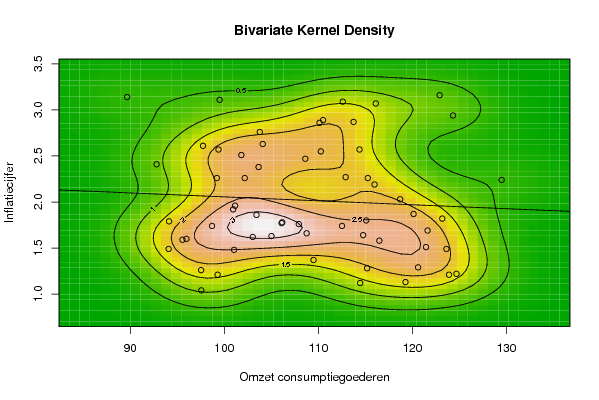
| Title produced by software | Bivariate Kernel Density Estimation | ||||||||||||||||||||||||||||||||||||||||||||
| Date of computation | Fri, 07 Nov 2008 03:38:01 -0700 | ||||||||||||||||||||||||||||||||||||||||||||
| Cite this page as follows | Statistical Computations at FreeStatistics.org, Office for Research Development and Education, URL https://freestatistics.org/blog/index.php?v=date/2008/Nov/07/t1226054348ayp62vxlkgti1w7.htm/, Retrieved Sun, 19 May 2024 06:30:56 +0000 | ||||||||||||||||||||||||||||||||||||||||||||
| Statistical Computations at FreeStatistics.org, Office for Research Development and Education, URL https://freestatistics.org/blog/index.php?pk=22467, Retrieved Sun, 19 May 2024 06:30:56 +0000 | |||||||||||||||||||||||||||||||||||||||||||||
| QR Codes: | |||||||||||||||||||||||||||||||||||||||||||||
|
| |||||||||||||||||||||||||||||||||||||||||||||
| Original text written by user: | |||||||||||||||||||||||||||||||||||||||||||||
| IsPrivate? | No (this computation is public) | ||||||||||||||||||||||||||||||||||||||||||||
| User-defined keywords | |||||||||||||||||||||||||||||||||||||||||||||
| Estimated Impact | 272 | ||||||||||||||||||||||||||||||||||||||||||||
Tree of Dependent Computations | |||||||||||||||||||||||||||||||||||||||||||||
| Family? (F = Feedback message, R = changed R code, M = changed R Module, P = changed Parameters, D = changed Data) | |||||||||||||||||||||||||||||||||||||||||||||
| F [Bivariate Kernel Density Estimation] [Various EDA topic...] [2008-11-07 10:38:01] [55ca0ca4a201c9689dcf5fae352c92eb] [Current] F RMPD [Trivariate Scatterplots] [Various EDA topic...] [2008-11-07 10:42:57] [e5d91604aae608e98a8ea24759233f66] F RMPD [Partial Correlation] [Various EDA topic...] [2008-11-07 10:48:55] [e5d91604aae608e98a8ea24759233f66] F RMPD [Box-Cox Linearity Plot] [Various EDA topic...] [2008-11-07 11:06:19] [e5d91604aae608e98a8ea24759233f66] F RM D [Box-Cox Normality Plot] [Various EDA topic...] [2008-11-10 11:55:49] [e5d91604aae608e98a8ea24759233f66] F RMPD [Maximum-likelihood Fitting - Normal Distribution] [Various EDA topic...] [2008-11-10 12:02:10] [e5d91604aae608e98a8ea24759233f66] - RMPD [Testing Variance - Critical Value (Region)] [Various types of ...] [2008-11-10 12:36:06] [e5d91604aae608e98a8ea24759233f66] - P [Testing Variance - Critical Value (Region)] [Various types of ...] [2008-11-10 12:44:47] [e5d91604aae608e98a8ea24759233f66] - RMPD [Notched Boxplots] [Various types of ...] [2008-11-10 13:05:18] [e5d91604aae608e98a8ea24759233f66] - RMPD [Testing Variance - p-value (probability)] [Various types of ...] [2008-11-10 12:39:28] [e5d91604aae608e98a8ea24759233f66] - RMPD [Kendall tau Correlation Matrix] [Various EDA topic...] [2008-11-07 11:03:18] [e5d91604aae608e98a8ea24759233f66] F RMPD [Testing Mean with known Variance - Critical Value] [Case - Q1] [2008-11-07 11:22:19] [e5d91604aae608e98a8ea24759233f66] F RM [Testing Mean with known Variance - p-value] [Case - Q2] [2008-11-07 11:40:30] [e5d91604aae608e98a8ea24759233f66] F RM [Testing Mean with known Variance - Type II Error] [Case - Q3] [2008-11-07 11:49:06] [e5d91604aae608e98a8ea24759233f66] F RM [Testing Mean with known Variance - Sample Size] [Case - Q4] [2008-11-07 11:55:44] [e5d91604aae608e98a8ea24759233f66] F RM [Testing Population Mean with known Variance - Confidence Interval] [Case - Q5] [2008-11-07 12:04:51] [e5d91604aae608e98a8ea24759233f66] - RM [Testing Sample Mean with known Variance - Confidence Interval] [Case - Q6] [2008-11-07 12:10:38] [e5d91604aae608e98a8ea24759233f66] F [Testing Sample Mean with known Variance - Confidence Interval] [Case - Q6.] [2008-11-07 12:17:52] [e5d91604aae608e98a8ea24759233f66] | |||||||||||||||||||||||||||||||||||||||||||||
| Feedback Forum | |||||||||||||||||||||||||||||||||||||||||||||
Post a new message | |||||||||||||||||||||||||||||||||||||||||||||
Dataset | |||||||||||||||||||||||||||||||||||||||||||||
| Dataseries X: | |||||||||||||||||||||||||||||||||||||||||||||
99,29 98,69 107,92 101,03 97,55 103,02 94,08 94,12 115,08 116,48 103,42 112,51 95,55 97,53 119,26 100,94 97,73 115,25 92,8 99,2 118,69 110,12 110,26 112,9 102,17 99,38 116,1 103,77 101,81 113,74 89,67 99,5 122,89 108,61 114,37 110,5 104,08 103,64 121,61 101,14 115,97 120,12 95,97 105,01 124,68 123,89 123,61 114,76 108,75 106,09 123,17 106,16 115,18 120,6 109,48 114,44 121,44 129,48 124,32 112,59 | |||||||||||||||||||||||||||||||||||||||||||||
| Dataseries Y: | |||||||||||||||||||||||||||||||||||||||||||||
1,21 1,74 1,76 1,48 1,04 1,62 1,49 1,79 1,8 1,58 1,86 1,74 1,59 1,26 1,13 1,92 2,61 2,26 2,41 2,26 2,03 2,86 2,55 2,27 2,26 2,57 3,07 2,76 2,51 2,87 3,14 3,11 3,16 2,47 2,57 2,89 2,63 2,38 1,69 1,96 2,19 1,87 1,6 1,63 1,22 1,21 1,49 1,64 1,66 1,77 1,82 1,78 1,28 1,29 1,37 1,12 1,51 2,24 2,94 3,09 | |||||||||||||||||||||||||||||||||||||||||||||
Tables (Output of Computation) | |||||||||||||||||||||||||||||||||||||||||||||
| |||||||||||||||||||||||||||||||||||||||||||||
Figures (Output of Computation) | |||||||||||||||||||||||||||||||||||||||||||||
Input Parameters & R Code | |||||||||||||||||||||||||||||||||||||||||||||
| Parameters (Session): | |||||||||||||||||||||||||||||||||||||||||||||
| par1 = 50 ; par2 = 50 ; par3 = 0 ; par4 = 0 ; par5 = 0 ; par6 = Y ; par7 = Y ; | |||||||||||||||||||||||||||||||||||||||||||||
| Parameters (R input): | |||||||||||||||||||||||||||||||||||||||||||||
| par1 = 50 ; par2 = 50 ; par3 = 0 ; par4 = 0 ; par5 = 0 ; par6 = Y ; par7 = Y ; | |||||||||||||||||||||||||||||||||||||||||||||
| R code (references can be found in the software module): | |||||||||||||||||||||||||||||||||||||||||||||
par1 <- as(par1,'numeric') | |||||||||||||||||||||||||||||||||||||||||||||