Free Statistics
of Irreproducible Research!
Description of Statistical Computation | |||||||||||||||||||||
|---|---|---|---|---|---|---|---|---|---|---|---|---|---|---|---|---|---|---|---|---|---|
| Author's title | |||||||||||||||||||||
| Author | *The author of this computation has been verified* | ||||||||||||||||||||
| R Software Module | rwasp_meanplot.wasp | ||||||||||||||||||||
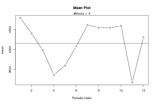
| Title produced by software | Mean Plot | ||||||||||||||||||||
| Date of computation | Wed, 05 Nov 2008 11:47:04 -0700 | ||||||||||||||||||||
| Cite this page as follows | Statistical Computations at FreeStatistics.org, Office for Research Development and Education, URL https://freestatistics.org/blog/index.php?v=date/2008/Nov/05/t1225910920vigchpi6o585bhd.htm/, Retrieved Sun, 19 May 2024 08:47:56 +0000 | ||||||||||||||||||||
| Statistical Computations at FreeStatistics.org, Office for Research Development and Education, URL https://freestatistics.org/blog/index.php?pk=21885, Retrieved Sun, 19 May 2024 08:47:56 +0000 | |||||||||||||||||||||
| QR Codes: | |||||||||||||||||||||
|
| |||||||||||||||||||||
| Original text written by user: | |||||||||||||||||||||
| IsPrivate? | No (this computation is public) | ||||||||||||||||||||
| User-defined keywords | |||||||||||||||||||||
| Estimated Impact | 188 | ||||||||||||||||||||
Tree of Dependent Computations | |||||||||||||||||||||
| Family? (F = Feedback message, R = changed R code, M = changed R Module, P = changed Parameters, D = changed Data) | |||||||||||||||||||||
| F [Mean Plot] [workshop 3] [2007-10-26 12:14:28] [e9ffc5de6f8a7be62f22b142b5b6b1a8] F R PD [Mean Plot] [vraag 2] [2008-10-29 19:00:24] [c45c87b96bbf32ffc2144fc37d767b2e] F R P [Mean Plot] [vraag 4] [2008-10-29 22:25:49] [c45c87b96bbf32ffc2144fc37d767b2e] F R PD [Mean Plot] [taak 5] [2008-10-30 06:53:19] [c45c87b96bbf32ffc2144fc37d767b2e] - P [Mean Plot] [herberekening] [2008-11-05 18:47:04] [3dc594a6c62226e1e98766c4d385bfaa] [Current] | |||||||||||||||||||||
| Feedback Forum | |||||||||||||||||||||
Post a new message | |||||||||||||||||||||
Dataset | |||||||||||||||||||||
| Dataseries X: | |||||||||||||||||||||
4348 3603 2700 2640 2916 3180 4151 4023 3431 3874 2617 3580 5267 3832 3441 3228 3397 3971 4625 4486 4131 4686 3174 4282 4209 4158 3936 3149 3623 4230 4443 4810 4853 5050 3553 4674 5412 5131 4856 3980 4431 4606 5352 4640 5170 4824 3280 4706 4909 5092 4911 3824 4214 4449 4486 4777 5132 4522 3295 4281 4590 4623 4075 3398 3029 | |||||||||||||||||||||
Tables (Output of Computation) | |||||||||||||||||||||
| |||||||||||||||||||||
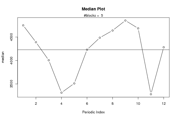
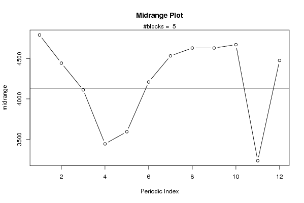
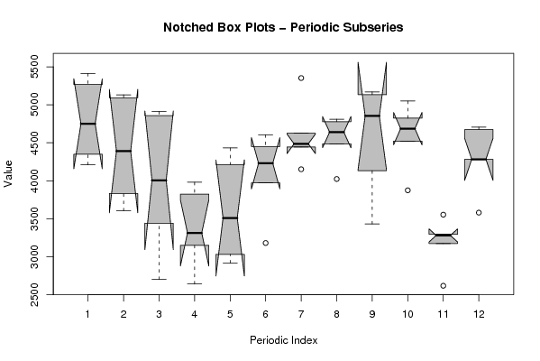
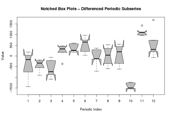
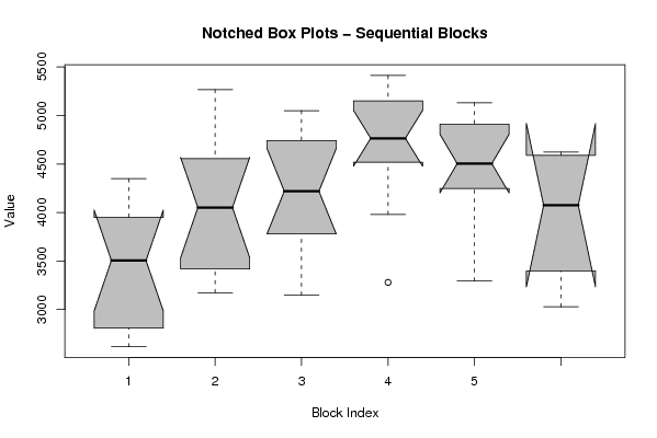
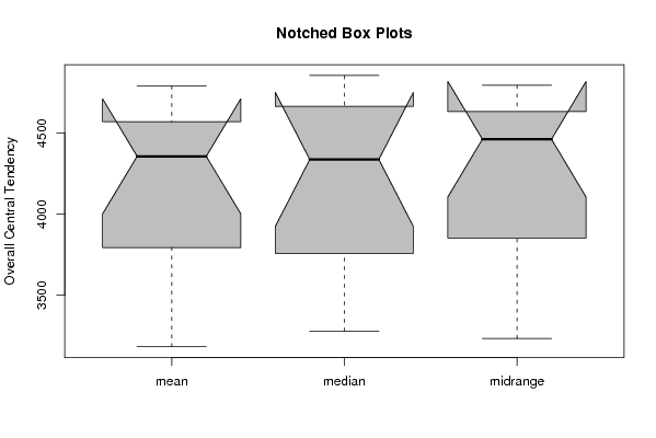
Figures (Output of Computation) | |||||||||||||||||||||
Input Parameters & R Code | |||||||||||||||||||||
| Parameters (Session): | |||||||||||||||||||||
| par1 = 12 ; | |||||||||||||||||||||
| Parameters (R input): | |||||||||||||||||||||
| par1 = 12 ; | |||||||||||||||||||||
| R code (references can be found in the software module): | |||||||||||||||||||||
par1 <- as.numeric(par1) | |||||||||||||||||||||