Free Statistics
of Irreproducible Research!
Description of Statistical Computation | |||||||||||||||||||||
|---|---|---|---|---|---|---|---|---|---|---|---|---|---|---|---|---|---|---|---|---|---|
| Author's title | |||||||||||||||||||||
| Author | *The author of this computation has been verified* | ||||||||||||||||||||
| R Software Module | rwasp_meanplot.wasp | ||||||||||||||||||||
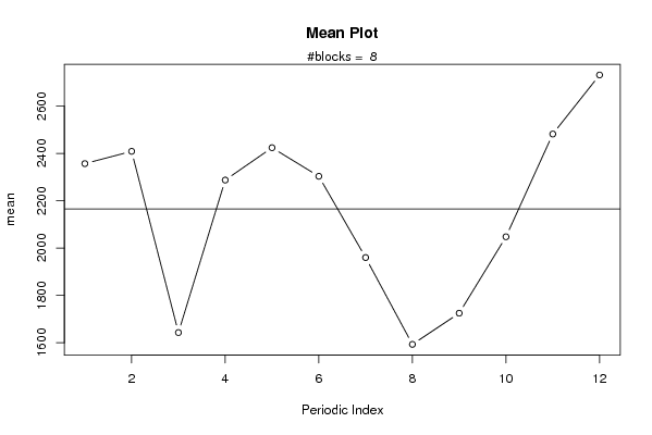
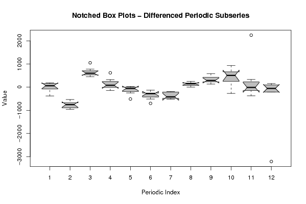
| Title produced by software | Mean Plot | ||||||||||||||||||||
| Date of computation | Mon, 03 Nov 2008 16:49:23 -0700 | ||||||||||||||||||||
| Cite this page as follows | Statistical Computations at FreeStatistics.org, Office for Research Development and Education, URL https://freestatistics.org/blog/index.php?v=date/2008/Nov/04/t1225756219g4f4sfq70j51nvt.htm/, Retrieved Sun, 19 May 2024 06:04:55 +0000 | ||||||||||||||||||||
| Statistical Computations at FreeStatistics.org, Office for Research Development and Education, URL https://freestatistics.org/blog/index.php?pk=21409, Retrieved Sun, 19 May 2024 06:04:55 +0000 | |||||||||||||||||||||
| QR Codes: | |||||||||||||||||||||
|
| |||||||||||||||||||||
| Original text written by user: | |||||||||||||||||||||
| IsPrivate? | No (this computation is public) | ||||||||||||||||||||
| User-defined keywords | |||||||||||||||||||||
| Estimated Impact | 186 | ||||||||||||||||||||
Tree of Dependent Computations | |||||||||||||||||||||
| Family? (F = Feedback message, R = changed R code, M = changed R Module, P = changed Parameters, D = changed Data) | |||||||||||||||||||||
| - [Mean Plot] [Mean Plot - Werke...] [2008-11-03 23:49:23] [7957bb37a64ed417bbed8444b0b0ea8a] [Current] F P [Mean Plot] [Mean Plot - Werke...] [2008-11-03 23:57:08] [fce9014b1ad8484790f3b34d6ba09f7b] - [Mean Plot] [] [2008-11-10 11:38:57] [888addc516c3b812dd7be4bd54caa358] | |||||||||||||||||||||
| Feedback Forum | |||||||||||||||||||||
Post a new message | |||||||||||||||||||||
Dataset | |||||||||||||||||||||
| Dataseries X: | |||||||||||||||||||||
2752 2373 1415 2466 2318 2346 1644 1421 1423 1930 2694 4938 1727 1899 1364 1992 2051 2082 1746 1271 1363 1664 2179 2305 2098 2231 1407 1966 2293 2045 1532 1333 1583 1712 2641 2267 2126 2231 1517 2010 2628 2115 1829 1636 1787 2122 2620 2555 2337 2524 1801 2417 2389 2267 2135 1760 1905 2176 2344 2673 2766 2785 2003 2588 2739 2703 2464 1974 2164 2385 2936 2700 2855 2764 1808 2588 2600 2526 2259 1738 1902 2137 2460 2495 2525 2465 1828 2273 2377 2344 2071 1611 1671 2256 1983 1921 2027 | |||||||||||||||||||||
Tables (Output of Computation) | |||||||||||||||||||||
| |||||||||||||||||||||
Figures (Output of Computation) | |||||||||||||||||||||
Input Parameters & R Code | |||||||||||||||||||||
| Parameters (Session): | |||||||||||||||||||||
| par1 = 12 ; | |||||||||||||||||||||
| Parameters (R input): | |||||||||||||||||||||
| par1 = 12 ; | |||||||||||||||||||||
| R code (references can be found in the software module): | |||||||||||||||||||||
par1 <- as.numeric(par1) | |||||||||||||||||||||