Free Statistics
of Irreproducible Research!
Description of Statistical Computation | |||||||||||||||||||||
|---|---|---|---|---|---|---|---|---|---|---|---|---|---|---|---|---|---|---|---|---|---|
| Author's title | |||||||||||||||||||||
| Author | *The author of this computation has been verified* | ||||||||||||||||||||
| R Software Module | rwasp_meanplot.wasp | ||||||||||||||||||||
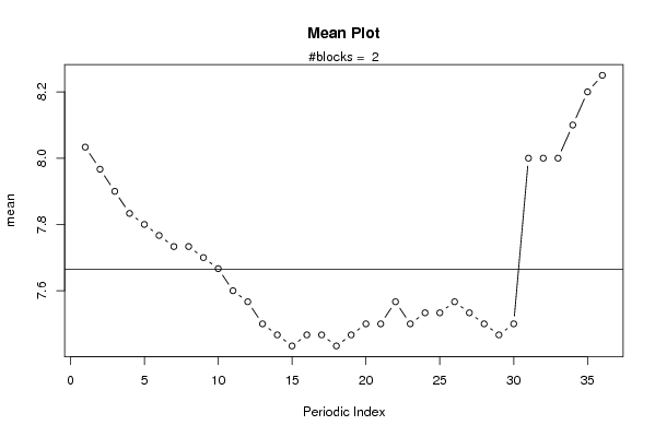
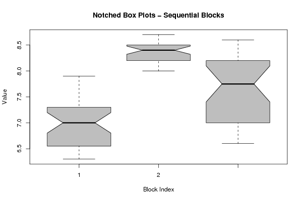
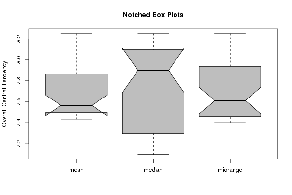
| Title produced by software | Mean Plot | ||||||||||||||||||||
| Date of computation | Mon, 03 Nov 2008 12:57:28 -0700 | ||||||||||||||||||||
| Cite this page as follows | Statistical Computations at FreeStatistics.org, Office for Research Development and Education, URL https://freestatistics.org/blog/index.php?v=date/2008/Nov/03/t1225742295mdj02zqexgs6ivt.htm/, Retrieved Sun, 13 Jul 2025 13:48:11 +0000 | ||||||||||||||||||||
| Statistical Computations at FreeStatistics.org, Office for Research Development and Education, URL https://freestatistics.org/blog/index.php?pk=21127, Retrieved Sun, 13 Jul 2025 13:48:11 +0000 | |||||||||||||||||||||
| QR Codes: | |||||||||||||||||||||
|
| |||||||||||||||||||||
| Original text written by user: | |||||||||||||||||||||
| IsPrivate? | No (this computation is public) | ||||||||||||||||||||
| User-defined keywords | |||||||||||||||||||||
| Estimated Impact | 208 | ||||||||||||||||||||
Tree of Dependent Computations | |||||||||||||||||||||
| Family? (F = Feedback message, R = changed R code, M = changed R Module, P = changed Parameters, D = changed Data) | |||||||||||||||||||||
| F [Mean Plot] [workshop 3] [2007-10-26 12:14:28] [e9ffc5de6f8a7be62f22b142b5b6b1a8] F PD [Mean Plot] [Hypothesis testin...] [2008-11-03 19:57:28] [4e8974eee929007194de34cbeefcb780] [Current] | |||||||||||||||||||||
| Feedback Forum | |||||||||||||||||||||
Post a new message | |||||||||||||||||||||
Dataset | |||||||||||||||||||||
| Dataseries X: | |||||||||||||||||||||
7,4 7,2 7,1 6,9 6,8 6,8 6,8 6,9 6,7 6,6 6,5 6,4 6,3 6,3 6,3 6,5 6,6 6,5 6,4 6,5 6,7 7,1 7,1 7,2 7,2 7,3 7,3 7,3 7,3 7,4 7,6 7,6 7,6 7,7 7,8 7,9 8,1 8,1 8,1 8,2 8,2 8,2 8,2 8,2 8,2 8,3 8,3 8,4 8,4 8,4 8,3 8 8 8,2 8,6 8,7 8,7 8,5 8,4 8,4 8,4 8,5 8,5 8,5 8,5 8,5 8,4 8,4 8,4 8,5 8,6 8,6 8,6 8,6 8,5 8,4 8,4 8,3 8,2 8,1 8,2 8,1 8 7,9 7,8 7,7 7,7 7,9 7,8 7,6 7,4 7,3 7,1 7,1 7 7 7 6,9 6,8 6,7 6,6 6,6 | |||||||||||||||||||||
Tables (Output of Computation) | |||||||||||||||||||||
| |||||||||||||||||||||
Figures (Output of Computation) | |||||||||||||||||||||
Input Parameters & R Code | |||||||||||||||||||||
| Parameters (Session): | |||||||||||||||||||||
| par1 = 36 ; | |||||||||||||||||||||
| Parameters (R input): | |||||||||||||||||||||
| par1 = 36 ; | |||||||||||||||||||||
| R code (references can be found in the software module): | |||||||||||||||||||||
par1 <- as.numeric(par1) | |||||||||||||||||||||