Free Statistics
of Irreproducible Research!
Description of Statistical Computation | |||||||||||||||||||||
|---|---|---|---|---|---|---|---|---|---|---|---|---|---|---|---|---|---|---|---|---|---|
| Author's title | |||||||||||||||||||||
| Author | *The author of this computation has been verified* | ||||||||||||||||||||
| R Software Module | rwasp_meanplot.wasp | ||||||||||||||||||||
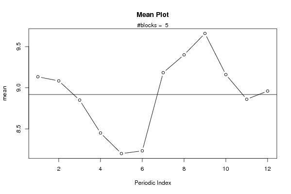
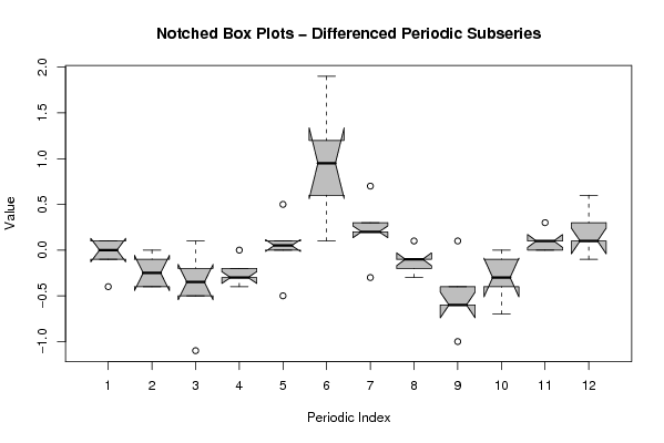
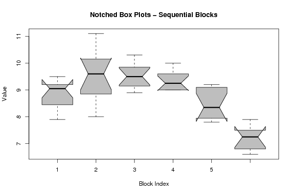
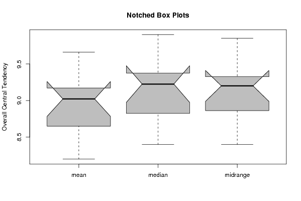
| Title produced by software | Mean Plot | ||||||||||||||||||||
| Date of computation | Mon, 03 Nov 2008 12:06:21 -0700 | ||||||||||||||||||||
| Cite this page as follows | Statistical Computations at FreeStatistics.org, Office for Research Development and Education, URL https://freestatistics.org/blog/index.php?v=date/2008/Nov/03/t12257392325yrp1d4ezngox9g.htm/, Retrieved Sun, 19 May 2024 11:11:32 +0000 | ||||||||||||||||||||
| Statistical Computations at FreeStatistics.org, Office for Research Development and Education, URL https://freestatistics.org/blog/index.php?pk=21001, Retrieved Sun, 19 May 2024 11:11:32 +0000 | |||||||||||||||||||||
| QR Codes: | |||||||||||||||||||||
|
| |||||||||||||||||||||
| Original text written by user: | |||||||||||||||||||||
| IsPrivate? | No (this computation is public) | ||||||||||||||||||||
| User-defined keywords | |||||||||||||||||||||
| Estimated Impact | 194 | ||||||||||||||||||||
Tree of Dependent Computations | |||||||||||||||||||||
| Family? (F = Feedback message, R = changed R code, M = changed R Module, P = changed Parameters, D = changed Data) | |||||||||||||||||||||
| F [Univariate Explorative Data Analysis] [Investigating dis...] [2007-10-22 19:45:25] [b9964c45117f7aac638ab9056d451faa] F D [Univariate Explorative Data Analysis] [Q7 tijdreeks werk...] [2008-10-27 16:45:31] [7d3039e6253bb5fb3b26df1537d500b4] F RMPD [Mean Plot] [Task 5 mean plot ...] [2008-11-03 19:06:21] [35348cd8592af0baf5f138bd59921307] [Current] | |||||||||||||||||||||
| Feedback Forum | |||||||||||||||||||||
Post a new message | |||||||||||||||||||||
Dataset | |||||||||||||||||||||
| Dataseries X: | |||||||||||||||||||||
9,0 9,1 8,7 8,2 7,9 7,9 9,1 9,4 9,5 9,1 9,0 9,3 9,9 9,8 9,4 8,3 8,0 8,5 10,4 11,1 10,9 9,9 9,2 9,2 9,5 9,6 9,5 9,1 8,9 9,0 10,1 10,3 10,2 9,6 9,2 9,3 9,4 9,4 9,2 9,0 9,0 9,0 9,8 10,0 9,9 9,3 9,0 9,0 9,1 9,1 9,1 9,2 8,8 8,3 8,4 8,1 7,8 7,9 7,9 8,0 7,9 7,5 7,2 6,9 6,6 6,7 7,3 7,5 | |||||||||||||||||||||
Tables (Output of Computation) | |||||||||||||||||||||
| |||||||||||||||||||||
Figures (Output of Computation) | |||||||||||||||||||||
Input Parameters & R Code | |||||||||||||||||||||
| Parameters (Session): | |||||||||||||||||||||
| par1 = 12 ; | |||||||||||||||||||||
| Parameters (R input): | |||||||||||||||||||||
| par1 = 12 ; | |||||||||||||||||||||
| R code (references can be found in the software module): | |||||||||||||||||||||
par1 <- as.numeric(par1) | |||||||||||||||||||||