Free Statistics
of Irreproducible Research!
Description of Statistical Computation | |||||||||||||||||||||
|---|---|---|---|---|---|---|---|---|---|---|---|---|---|---|---|---|---|---|---|---|---|
| Author's title | |||||||||||||||||||||
| Author | *The author of this computation has been verified* | ||||||||||||||||||||
| R Software Module | rwasp_meanplot.wasp | ||||||||||||||||||||
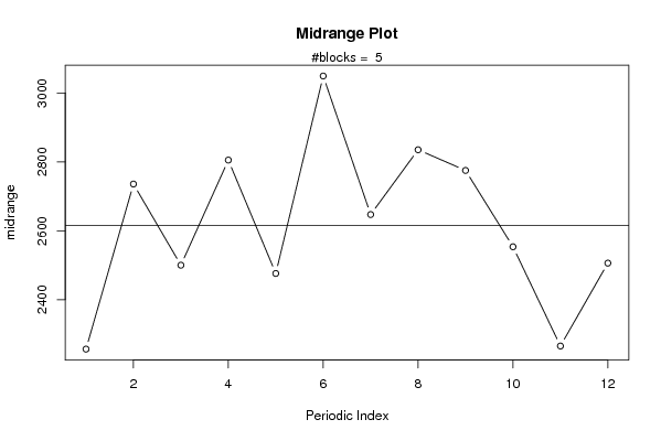
| Title produced by software | Mean Plot | ||||||||||||||||||||
| Date of computation | Mon, 03 Nov 2008 02:10:45 -0700 | ||||||||||||||||||||
| Cite this page as follows | Statistical Computations at FreeStatistics.org, Office for Research Development and Education, URL https://freestatistics.org/blog/index.php?v=date/2008/Nov/03/t1225703650kz9aqttkcgpjjh7.htm/, Retrieved Sun, 19 May 2024 12:40:57 +0000 | ||||||||||||||||||||
| Statistical Computations at FreeStatistics.org, Office for Research Development and Education, URL https://freestatistics.org/blog/index.php?pk=20767, Retrieved Sun, 19 May 2024 12:40:57 +0000 | |||||||||||||||||||||
| QR Codes: | |||||||||||||||||||||
|
| |||||||||||||||||||||
| Original text written by user: | |||||||||||||||||||||
| IsPrivate? | No (this computation is public) | ||||||||||||||||||||
| User-defined keywords | |||||||||||||||||||||
| Estimated Impact | 196 | ||||||||||||||||||||
Tree of Dependent Computations | |||||||||||||||||||||
| Family? (F = Feedback message, R = changed R code, M = changed R Module, P = changed Parameters, D = changed Data) | |||||||||||||||||||||
| F [Mean Plot] [workshop 3] [2007-10-26 12:14:28] [e9ffc5de6f8a7be62f22b142b5b6b1a8] - R D [Mean Plot] [Opdracht 4 task 5...] [2008-11-03 09:10:45] [73ec5abea95a9c3c8c3a1ac44cab1f72] [Current] - [Mean Plot] [Opdracht 4 task 5...] [2008-11-03 09:18:51] [1848c1c05ef454c234bcbe26cf08badc] - [Mean Plot] [Opdracht 4 task 5...] [2008-11-03 09:24:26] [1848c1c05ef454c234bcbe26cf08badc] | |||||||||||||||||||||
| Feedback Forum | |||||||||||||||||||||
Post a new message | |||||||||||||||||||||
Dataset | |||||||||||||||||||||
| Dataseries X: | |||||||||||||||||||||
2490 3266 3475 3127 2955 3870 2852 3142 3029 3180 2560 2733 2452 2553 2777 2520 2318 2873 2311 2395 2099 2268 2316 2181 2175 2627 2578 3090 2634 3225 2938 3174 3350 2588 2061 2691 2061 2918 2223 2651 2379 3146 2883 2768 3258 2839 2470 5072 1463 1600 2203 2013 2169 2640 2411 2528 2292 1988 1774 2279 | |||||||||||||||||||||
Tables (Output of Computation) | |||||||||||||||||||||
| |||||||||||||||||||||
Figures (Output of Computation) | |||||||||||||||||||||
Input Parameters & R Code | |||||||||||||||||||||
| Parameters (Session): | |||||||||||||||||||||
| par1 = 12 ; | |||||||||||||||||||||
| Parameters (R input): | |||||||||||||||||||||
| par1 = 12 ; | |||||||||||||||||||||
| R code (references can be found in the software module): | |||||||||||||||||||||
par1 <- as.numeric(par1) | |||||||||||||||||||||