Free Statistics
of Irreproducible Research!
Description of Statistical Computation | |||||||||||||||||||||
|---|---|---|---|---|---|---|---|---|---|---|---|---|---|---|---|---|---|---|---|---|---|
| Author's title | |||||||||||||||||||||
| Author | *Unverified author* | ||||||||||||||||||||
| R Software Module | rwasp_meanplot.wasp | ||||||||||||||||||||
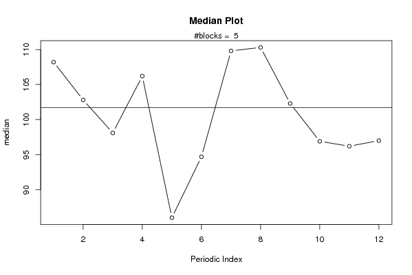
| Title produced by software | Mean Plot | ||||||||||||||||||||
| Date of computation | Sun, 02 Nov 2008 14:48:27 -0700 | ||||||||||||||||||||
| Cite this page as follows | Statistical Computations at FreeStatistics.org, Office for Research Development and Education, URL https://freestatistics.org/blog/index.php?v=date/2008/Nov/02/t1225662672c4h9fo0ds189zgb.htm/, Retrieved Sun, 19 May 2024 11:31:34 +0000 | ||||||||||||||||||||
| Statistical Computations at FreeStatistics.org, Office for Research Development and Education, URL https://freestatistics.org/blog/index.php?pk=20725, Retrieved Sun, 19 May 2024 11:31:34 +0000 | |||||||||||||||||||||
| QR Codes: | |||||||||||||||||||||
|
| |||||||||||||||||||||
| Original text written by user: | |||||||||||||||||||||
| IsPrivate? | No (this computation is public) | ||||||||||||||||||||
| User-defined keywords | |||||||||||||||||||||
| Estimated Impact | 157 | ||||||||||||||||||||
Tree of Dependent Computations | |||||||||||||||||||||
| Family? (F = Feedback message, R = changed R code, M = changed R Module, P = changed Parameters, D = changed Data) | |||||||||||||||||||||
| F [Notched Boxplots] [workshop 3] [2007-10-26 13:31:48] [e9ffc5de6f8a7be62f22b142b5b6b1a8] F D [Notched Boxplots] [task 2] [2008-11-02 15:47:37] [73d6180dc45497329efd1b6934a84aba] F PD [Notched Boxplots] [Task 2] [2008-11-02 19:05:58] [6816386b1f3c2f6c0c9f2aa1e5bc9362] - RMPD [Mean Plot] [task 2 (total pro...] [2008-11-02 21:48:27] [81dc0ee785f23261ccd6abf7aef76c2a] [Current] | |||||||||||||||||||||
| Feedback Forum | |||||||||||||||||||||
Post a new message | |||||||||||||||||||||
Dataset | |||||||||||||||||||||
| Dataseries X: | |||||||||||||||||||||
110,40 96,40 101,90 106,20 81,00 94,70 101,00 109,40 102,30 90,70 96,20 96,10 106,00 103,10 102,00 104,70 86,00 92,10 106,90 112,60 101,70 92,00 97,40 97,00 105,40 102,70 98,10 104,50 87,40 89,90 109,80 111,70 98,60 96,90 95,10 97,00 112,70 102,90 97,40 111,40 87,40 96,80 114,10 110,30 103,90 101,60 94,60 95,90 104,70 102,80 98,10 113,90 80,90 95,70 113,20 105,90 108,80 102,30 99,00 100,70 115,50 | |||||||||||||||||||||
Tables (Output of Computation) | |||||||||||||||||||||
| |||||||||||||||||||||
Figures (Output of Computation) | |||||||||||||||||||||
Input Parameters & R Code | |||||||||||||||||||||
| Parameters (Session): | |||||||||||||||||||||
| par1 = 12 ; | |||||||||||||||||||||
| Parameters (R input): | |||||||||||||||||||||
| par1 = 12 ; | |||||||||||||||||||||
| R code (references can be found in the software module): | |||||||||||||||||||||
par1 <- as.numeric(par1) | |||||||||||||||||||||