Free Statistics
of Irreproducible Research!
Description of Statistical Computation | |||||||||||||||||||||
|---|---|---|---|---|---|---|---|---|---|---|---|---|---|---|---|---|---|---|---|---|---|
| Author's title | |||||||||||||||||||||
| Author | *The author of this computation has been verified* | ||||||||||||||||||||
| R Software Module | rwasp_meanplot.wasp | ||||||||||||||||||||
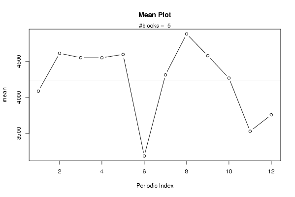
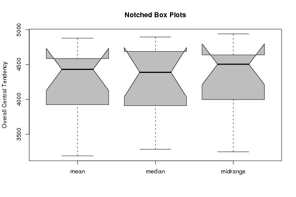
| Title produced by software | Mean Plot | ||||||||||||||||||||
| Date of computation | Sun, 02 Nov 2008 09:28:53 -0700 | ||||||||||||||||||||
| Cite this page as follows | Statistical Computations at FreeStatistics.org, Office for Research Development and Education, URL https://freestatistics.org/blog/index.php?v=date/2008/Nov/02/t1225643384kx5ktqknvb007x6.htm/, Retrieved Sun, 19 May 2024 09:17:43 +0000 | ||||||||||||||||||||
| Statistical Computations at FreeStatistics.org, Office for Research Development and Education, URL https://freestatistics.org/blog/index.php?pk=20643, Retrieved Sun, 19 May 2024 09:17:43 +0000 | |||||||||||||||||||||
| QR Codes: | |||||||||||||||||||||
|
| |||||||||||||||||||||
| Original text written by user: | |||||||||||||||||||||
| IsPrivate? | No (this computation is public) | ||||||||||||||||||||
| User-defined keywords | |||||||||||||||||||||
| Estimated Impact | 144 | ||||||||||||||||||||
Tree of Dependent Computations | |||||||||||||||||||||
| Family? (F = Feedback message, R = changed R code, M = changed R Module, P = changed Parameters, D = changed Data) | |||||||||||||||||||||
| F [Univariate Data Series] [blog 1e tijdreeks...] [2008-10-13 19:23:31] [7173087adebe3e3a714c80ea2417b3eb] - PD [Univariate Data Series] [tijdreeksen opnie...] [2008-10-19 17:21:24] [7173087adebe3e3a714c80ea2417b3eb] - PD [Univariate Data Series] [tijdreeksen opnie...] [2008-10-19 19:01:42] [7173087adebe3e3a714c80ea2417b3eb] - RMP [Mean Plot] [mean plot reeks 3] [2008-11-02 16:28:53] [95d95b0e883740fcbc85e18ec42dcafb] [Current] | |||||||||||||||||||||
| Feedback Forum | |||||||||||||||||||||
Post a new message | |||||||||||||||||||||
Dataset | |||||||||||||||||||||
| Dataseries X: | |||||||||||||||||||||
3180 4151 4023 3431 3874 2617 3580 5267 3832 3441 3228 3397 3971 4625 4486 4131 4686 3174 4282 4209 4159 3936 3153 3620 4227 4441 4808 4850 5040 3546 4669 5410 5134 4864 3999 4459 4622 5360 4658 5173 4845 3325 4720 4895 5071 4895 3805 4187 4435 4475 4774 5161 4529 3284 4303 4610 4691 4200 3471 3132 | |||||||||||||||||||||
Tables (Output of Computation) | |||||||||||||||||||||
| |||||||||||||||||||||
Figures (Output of Computation) | |||||||||||||||||||||
Input Parameters & R Code | |||||||||||||||||||||
| Parameters (Session): | |||||||||||||||||||||
| par1 = 12 ; | |||||||||||||||||||||
| Parameters (R input): | |||||||||||||||||||||
| par1 = 12 ; | |||||||||||||||||||||
| R code (references can be found in the software module): | |||||||||||||||||||||
par1 <- as.numeric(par1) | |||||||||||||||||||||