Free Statistics
of Irreproducible Research!
Description of Statistical Computation | |||||||||||||||||||||
|---|---|---|---|---|---|---|---|---|---|---|---|---|---|---|---|---|---|---|---|---|---|
| Author's title | |||||||||||||||||||||
| Author | *The author of this computation has been verified* | ||||||||||||||||||||
| R Software Module | rwasp_meanplot.wasp | ||||||||||||||||||||
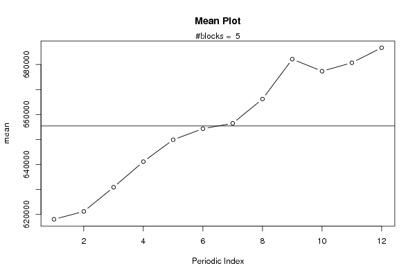
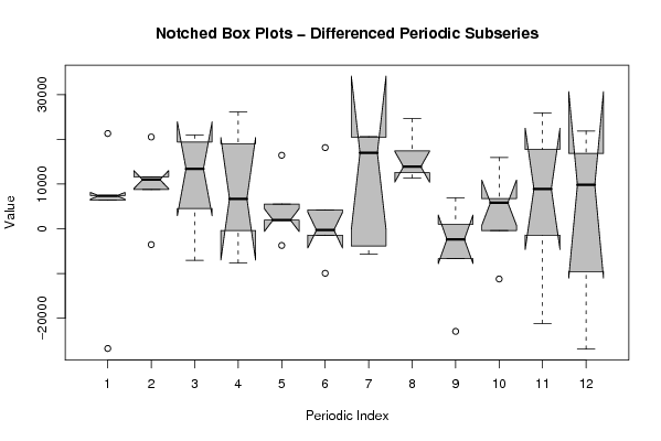
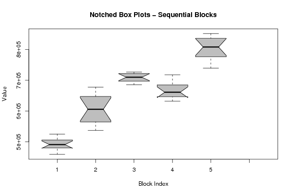
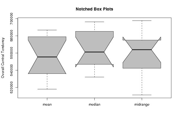
| Title produced by software | Mean Plot | ||||||||||||||||||||
| Date of computation | Sun, 02 Nov 2008 09:22:21 -0700 | ||||||||||||||||||||
| Cite this page as follows | Statistical Computations at FreeStatistics.org, Office for Research Development and Education, URL https://freestatistics.org/blog/index.php?v=date/2008/Nov/02/t1225642983459aja24m6q02ug.htm/, Retrieved Sun, 19 May 2024 11:38:04 +0000 | ||||||||||||||||||||
| Statistical Computations at FreeStatistics.org, Office for Research Development and Education, URL https://freestatistics.org/blog/index.php?pk=20640, Retrieved Sun, 19 May 2024 11:38:04 +0000 | |||||||||||||||||||||
| QR Codes: | |||||||||||||||||||||
|
| |||||||||||||||||||||
| Original text written by user: | |||||||||||||||||||||
| IsPrivate? | No (this computation is public) | ||||||||||||||||||||
| User-defined keywords | |||||||||||||||||||||
| Estimated Impact | 184 | ||||||||||||||||||||
Tree of Dependent Computations | |||||||||||||||||||||
| Family? (F = Feedback message, R = changed R code, M = changed R Module, P = changed Parameters, D = changed Data) | |||||||||||||||||||||
| F [Notched Boxplots] [workshop 3] [2007-10-26 13:31:48] [e9ffc5de6f8a7be62f22b142b5b6b1a8] F RMPD [Mean Plot] [workshop 4 deel 1...] [2008-10-31 09:40:26] [077ffec662d24c06be4c491541a44245] F [Mean Plot] [] [2008-11-01 13:19:15] [4c8dfb519edec2da3492d7e6be9a5685] F D [Mean Plot] [] [2008-11-01 14:24:03] [4c8dfb519edec2da3492d7e6be9a5685] - D [Mean Plot] [task 5] [2008-11-02 16:22:21] [e81ac192d6ae6d77191d83851a692999] [Current] | |||||||||||||||||||||
| Feedback Forum | |||||||||||||||||||||
Post a new message | |||||||||||||||||||||
Dataset | |||||||||||||||||||||
| Dataseries X: | |||||||||||||||||||||
459191 466617 477604 482132 488837 490761 495016 491156 502519 509405 516184 525109 536953 543315 554950 574343 600423 605963 605672 626140 650740 644045 659971 677720 685500 692880 713398 726815 726448 722721 712776 707154 721030 698097 697694 696268 669371 642615 639078 632034 651048 652996 651578 672179 684741 685734 691557 717499 739340 760643 769425 790364 782748 799182 817333 834295 851736 849382 838158 817005 | |||||||||||||||||||||
Tables (Output of Computation) | |||||||||||||||||||||
| |||||||||||||||||||||
Figures (Output of Computation) | |||||||||||||||||||||
Input Parameters & R Code | |||||||||||||||||||||
| Parameters (Session): | |||||||||||||||||||||
| par1 = 12 ; | |||||||||||||||||||||
| Parameters (R input): | |||||||||||||||||||||
| par1 = 12 ; | |||||||||||||||||||||
| R code (references can be found in the software module): | |||||||||||||||||||||
par1 <- as.numeric(par1) | |||||||||||||||||||||