Free Statistics
of Irreproducible Research!
Description of Statistical Computation | |||||||||||||||||||||
|---|---|---|---|---|---|---|---|---|---|---|---|---|---|---|---|---|---|---|---|---|---|
| Author's title | |||||||||||||||||||||
| Author | *The author of this computation has been verified* | ||||||||||||||||||||
| R Software Module | rwasp_meanplot.wasp | ||||||||||||||||||||
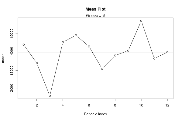
| Title produced by software | Mean Plot | ||||||||||||||||||||
| Date of computation | Sun, 02 Nov 2008 09:03:09 -0700 | ||||||||||||||||||||
| Cite this page as follows | Statistical Computations at FreeStatistics.org, Office for Research Development and Education, URL https://freestatistics.org/blog/index.php?v=date/2008/Nov/02/t1225641829amqpyknhswqdgly.htm/, Retrieved Sun, 19 May 2024 11:14:55 +0000 | ||||||||||||||||||||
| Statistical Computations at FreeStatistics.org, Office for Research Development and Education, URL https://freestatistics.org/blog/index.php?pk=20632, Retrieved Sun, 19 May 2024 11:14:55 +0000 | |||||||||||||||||||||
| QR Codes: | |||||||||||||||||||||
|
| |||||||||||||||||||||
| Original text written by user: | |||||||||||||||||||||
| IsPrivate? | No (this computation is public) | ||||||||||||||||||||
| User-defined keywords | |||||||||||||||||||||
| Estimated Impact | 193 | ||||||||||||||||||||
Tree of Dependent Computations | |||||||||||||||||||||
| Family? (F = Feedback message, R = changed R code, M = changed R Module, P = changed Parameters, D = changed Data) | |||||||||||||||||||||
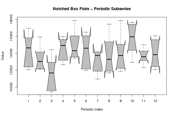
| F [Notched Boxplots] [workshop 3] [2007-10-26 13:31:48] [e9ffc5de6f8a7be62f22b142b5b6b1a8] F RMPD [Mean Plot] [workshop 4 deel 1...] [2008-10-31 09:40:26] [077ffec662d24c06be4c491541a44245] F [Mean Plot] [] [2008-11-01 13:19:15] [4c8dfb519edec2da3492d7e6be9a5685] F D [Mean Plot] [] [2008-11-01 14:24:03] [4c8dfb519edec2da3492d7e6be9a5685] F D [Mean Plot] [Task 5 - Bob Leysen] [2008-11-02 16:03:09] [0831954c833179c36e9320daee0825b5] [Current] F D [Mean Plot] [opdracht 4 task 5] [2008-11-03 17:56:26] [077ffec662d24c06be4c491541a44245] | |||||||||||||||||||||
| Feedback Forum | |||||||||||||||||||||
Post a new message | |||||||||||||||||||||
Dataset | |||||||||||||||||||||
| Dataseries X: | |||||||||||||||||||||
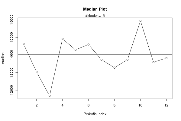
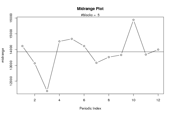
12055 12113 9617 12646 13581 12162 10970 11880 11888 12927 12300 12093 12381 12197 9455 13168 13428 11981 11885 11692 12234 14341 13131 12421 14286 12865 11160 14316 14389 14014 13419 12770 13316 15333 14243 13824 14963 13203 12199 15509 14200 15170 14058 13786 14148 16542 13588 15582 15803 14131 12923 15612 16034 16037 14038 15331 15038 17402 14993 16044 16930 15921 14417 15961 17852 16484 14216 17430 17840 17629 | |||||||||||||||||||||
Tables (Output of Computation) | |||||||||||||||||||||
| |||||||||||||||||||||
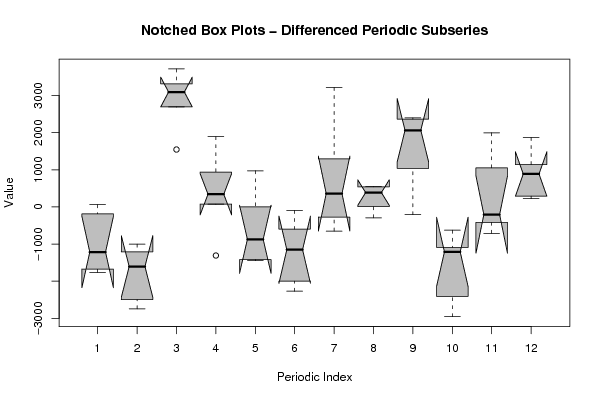
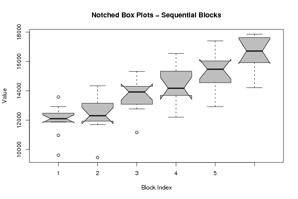
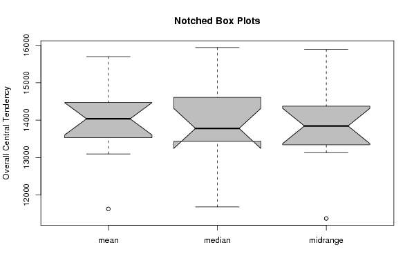
Figures (Output of Computation) | |||||||||||||||||||||
Input Parameters & R Code | |||||||||||||||||||||
| Parameters (Session): | |||||||||||||||||||||
| par1 = 12 ; | |||||||||||||||||||||
| Parameters (R input): | |||||||||||||||||||||
| par1 = 12 ; | |||||||||||||||||||||
| R code (references can be found in the software module): | |||||||||||||||||||||
par1 <- as.numeric(par1) | |||||||||||||||||||||