Free Statistics
of Irreproducible Research!
Description of Statistical Computation | |||||||||||||||||||||
|---|---|---|---|---|---|---|---|---|---|---|---|---|---|---|---|---|---|---|---|---|---|
| Author's title | |||||||||||||||||||||
| Author | *The author of this computation has been verified* | ||||||||||||||||||||
| R Software Module | rwasp_meanplot.wasp | ||||||||||||||||||||
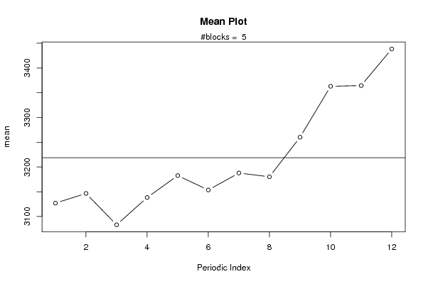
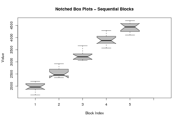
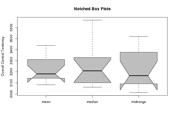
| Title produced by software | Mean Plot | ||||||||||||||||||||
| Date of computation | Sun, 02 Nov 2008 04:01:35 -0700 | ||||||||||||||||||||
| Cite this page as follows | Statistical Computations at FreeStatistics.org, Office for Research Development and Education, URL https://freestatistics.org/blog/index.php?v=date/2008/Nov/02/t1225623747n39erlp4qn61vxq.htm/, Retrieved Sun, 19 May 2024 08:53:11 +0000 | ||||||||||||||||||||
| Statistical Computations at FreeStatistics.org, Office for Research Development and Education, URL https://freestatistics.org/blog/index.php?pk=20491, Retrieved Sun, 19 May 2024 08:53:11 +0000 | |||||||||||||||||||||
| QR Codes: | |||||||||||||||||||||
|
| |||||||||||||||||||||
| Original text written by user: | |||||||||||||||||||||
| IsPrivate? | No (this computation is public) | ||||||||||||||||||||
| User-defined keywords | |||||||||||||||||||||
| Estimated Impact | 179 | ||||||||||||||||||||
Tree of Dependent Computations | |||||||||||||||||||||
| Family? (F = Feedback message, R = changed R code, M = changed R Module, P = changed Parameters, D = changed Data) | |||||||||||||||||||||
| - [Mean Plot] [Hypothesen taak 5...] [2008-10-31 11:04:33] [e5d91604aae608e98a8ea24759233f66] - D [Mean Plot] [Hypothesen taak 5...] [2008-11-02 11:01:35] [55ca0ca4a201c9689dcf5fae352c92eb] [Current] - D [Mean Plot] [Hypothesen deel 2...] [2008-11-02 12:35:43] [e5d91604aae608e98a8ea24759233f66] - D [Mean Plot] [Hypothesen deel 2...] [2008-11-02 12:37:14] [e5d91604aae608e98a8ea24759233f66] - D [Mean Plot] [Hypothesen deel 2...] [2008-11-02 12:38:35] [e5d91604aae608e98a8ea24759233f66] - D [Mean Plot] [Hypothesen deel 2...] [2008-11-02 12:40:28] [e5d91604aae608e98a8ea24759233f66] - D [Mean Plot] [Hypothesen deel 2...] [2008-11-02 12:41:47] [e5d91604aae608e98a8ea24759233f66] | |||||||||||||||||||||
| Feedback Forum | |||||||||||||||||||||
Post a new message | |||||||||||||||||||||
Dataset | |||||||||||||||||||||
| Dataseries X: | |||||||||||||||||||||
1946,81 1765,9 1635,25 1833,42 1910,43 1959,67 1969,6 2061,41 2093,48 2120,88 2174,56 2196,72 2350,44 2440,25 2408,64 2472,81 2407,6 2454,62 2448,05 2497,84 2645,64 2756,76 2849,27 2921,44 3080,58 3106,22 3119,31 3061,26 3097,31 3161,69 3257,16 3277,01 3295,32 3363,99 3494,17 3667,03 3813,06 3917,96 3895,51 3733,22 3801,06 3570,12 3701,61 3862,27 3970,1 4138,52 4199,75 4290,89 4443,91 4502,64 4356,98 4591,27 4696,96 4621,4 4562,84 4202,52 4296,49 4435,23 4105,18 4116,68 | |||||||||||||||||||||
Tables (Output of Computation) | |||||||||||||||||||||
| |||||||||||||||||||||
Figures (Output of Computation) | |||||||||||||||||||||
Input Parameters & R Code | |||||||||||||||||||||
| Parameters (Session): | |||||||||||||||||||||
| par1 = 12 ; | |||||||||||||||||||||
| Parameters (R input): | |||||||||||||||||||||
| par1 = 12 ; | |||||||||||||||||||||
| R code (references can be found in the software module): | |||||||||||||||||||||
par1 <- as.numeric(par1) | |||||||||||||||||||||