Free Statistics
of Irreproducible Research!
Description of Statistical Computation | ||||||||||||||||||||||||||
|---|---|---|---|---|---|---|---|---|---|---|---|---|---|---|---|---|---|---|---|---|---|---|---|---|---|---|
| Author's title | ||||||||||||||||||||||||||
| Author | *The author of this computation has been verified* | |||||||||||||||||||||||||
| R Software Module | rwasp_meanplot.wasp | |||||||||||||||||||||||||
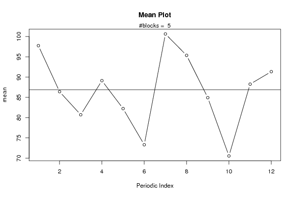
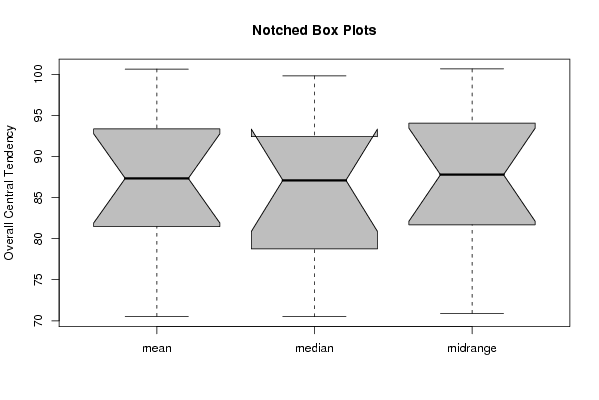
| Title produced by software | Mean Plot | |||||||||||||||||||||||||
| Date of computation | Sat, 01 Nov 2008 05:04:36 -0600 | |||||||||||||||||||||||||
| Cite this page as follows | Statistical Computations at FreeStatistics.org, Office for Research Development and Education, URL https://freestatistics.org/blog/index.php?v=date/2008/Nov/01/t1225537524excne2bplqi9q4v.htm/, Retrieved Sun, 19 May 2024 12:38:57 +0000 | |||||||||||||||||||||||||
| Statistical Computations at FreeStatistics.org, Office for Research Development and Education, URL https://freestatistics.org/blog/index.php?pk=20347, Retrieved Sun, 19 May 2024 12:38:57 +0000 | ||||||||||||||||||||||||||
| QR Codes: | ||||||||||||||||||||||||||
|
| ||||||||||||||||||||||||||
| Original text written by user: | ||||||||||||||||||||||||||
| IsPrivate? | No (this computation is public) | |||||||||||||||||||||||||
| User-defined keywords | ||||||||||||||||||||||||||
| Estimated Impact | 234 | |||||||||||||||||||||||||
Tree of Dependent Computations | ||||||||||||||||||||||||||
| Family? (F = Feedback message, R = changed R code, M = changed R Module, P = changed Parameters, D = changed Data) | ||||||||||||||||||||||||||
| F [Mean Plot] [workshop 3] [2007-10-26 12:14:28] [e9ffc5de6f8a7be62f22b142b5b6b1a8] F D [Mean Plot] [Hypotheses Testin...] [2008-11-01 11:04:36] [dafd615cb3e0decc017580d68ecea30a] [Current] F R [Mean Plot] [Testing Hypothese...] [2008-11-01 14:30:28] [33f4701c7363e8b81858dafbf0350eed] F [Mean Plot] [T4] [2008-11-03 18:59:42] [b187fac1a1b0cb3920f54366df47fea3] - [Mean Plot] [task 4 , I] [2008-11-03 20:38:39] [1e82cb4c98d4057b5653dbe7a07f2cda] F [Mean Plot] [task 4] [2008-11-03 23:01:48] [b641c14ac36cb6fee377f3b099dcac19] - [Mean Plot] [] [2008-11-09 19:44:34] [888addc516c3b812dd7be4bd54caa358] F D [Mean Plot] [Testing Hypothese...] [2008-11-01 15:12:37] [33f4701c7363e8b81858dafbf0350eed] F D [Mean Plot] [T5] [2008-11-03 19:05:19] [b187fac1a1b0cb3920f54366df47fea3] - [Mean Plot] [Task 5] [2008-11-03 20:50:18] [1e82cb4c98d4057b5653dbe7a07f2cda] F [Mean Plot] [task 5] [2008-11-03 23:06:08] [b641c14ac36cb6fee377f3b099dcac19] - [Mean Plot] [] [2008-11-09 19:54:39] [888addc516c3b812dd7be4bd54caa358] - [Mean Plot] [] [2008-11-09 19:54:39] [888addc516c3b812dd7be4bd54caa358] F [Mean Plot] [T1 - Q2] [2008-11-03 18:44:09] [b187fac1a1b0cb3920f54366df47fea3] F [Mean Plot] [q2] [2008-11-03 22:50:51] [b641c14ac36cb6fee377f3b099dcac19] - [Mean Plot] [] [2008-11-09 18:39:24] [888addc516c3b812dd7be4bd54caa358] | ||||||||||||||||||||||||||
| Feedback Forum | ||||||||||||||||||||||||||
Post a new message | ||||||||||||||||||||||||||
Dataset | ||||||||||||||||||||||||||
| Dataseries X: | ||||||||||||||||||||||||||
109.20 88.60 94.30 98.30 86.40 80.60 104.10 108.20 93.40 71.90 94.10 94.90 96.40 91.10 84.40 86.40 88.00 75.10 109.70 103.00 82.10 68.00 96.40 94.30 90.00 88.00 76.10 82.50 81.40 66.50 97.20 94.10 80.70 70.50 87.80 89.50 99.60 84.20 75.10 92.00 80.80 73.10 99.80 90.00 83.10 72.40 78.80 87.30 91.00 80.10 73.60 86.40 74.50 71.20 92.40 81.50 85.30 69.90 84.20 90.70 100.30 | ||||||||||||||||||||||||||
Tables (Output of Computation) | ||||||||||||||||||||||||||
| ||||||||||||||||||||||||||
Figures (Output of Computation) | ||||||||||||||||||||||||||
Input Parameters & R Code | ||||||||||||||||||||||||||
| Parameters (Session): | ||||||||||||||||||||||||||
| par1 = 12 ; | ||||||||||||||||||||||||||
| Parameters (R input): | ||||||||||||||||||||||||||
| par1 = 12 ; | ||||||||||||||||||||||||||
| R code (references can be found in the software module): | ||||||||||||||||||||||||||
par1 <- as.numeric(par1) | ||||||||||||||||||||||||||