Free Statistics

of Irreproducible Research!

Author's title

exponential smoothing gemiddelde consumptieprijzen mineraalwater - Rebecca ...

Author

*Unverified author*

R Software Module

rwasp_exponentialsmoothing.wasp

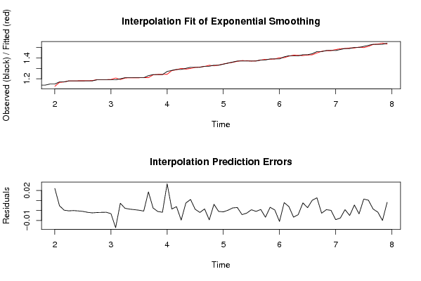
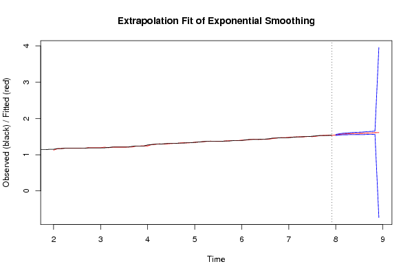
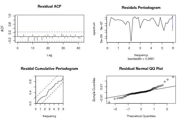
Title produced by software

Exponential Smoothing

Date of computation

Tue, 27 May 2008 12:54:41 -0600

Cite this page as follows

Statistical Computations at FreeStatistics.org, Office for Research Development and Education, URL https://freestatistics.org/blog/index.php?v=date/2008/May/27/t1211914613bqb3hvov8t0ncv2.htm/, Retrieved Mon, 20 May 2024 00:08:24 +0000

Statistical Computations at FreeStatistics.org, Office for Research Development and Education, URL https://freestatistics.org/blog/index.php?pk=13379, Retrieved Mon, 20 May 2024 00:08:24 +0000

QR Codes:

Paste this QR Code to cite your computation.

Original text written by user:

IsPrivate?

No (this computation is public)

User-defined keywords

Estimated Impact

179

Family? (F = Feedback message, R = changed R code, M = changed R Module, P = changed Parameters, D = changed Data)

-       [Exponential Smoothing] [exponential smoot...] [2008-05-27 18:54:41] [d41d8cd98f00b204e9800998ecf8427e] [Current]

Feedback Forum

Post a new message

Dataseries X:

Download CSV

Histogram

Boxplots

1,12
1,12
1,12
1,13
1,13
1,13
1,14
1,14
1,14
1,14
1,14
1,15
1,15
1,17
1,17
1,18
1,18
1,18
1,18
1,18
1,18
1,19
1,19
1,19
1,19
1,19
1,2
1,21
1,21
1,21
1,21
1,21
1,23
1,24
1,24
1,24
1,27
1,28
1,29
1,29
1,3
1,31
1,31
1,31
1,32
1,32
1,33
1,33
1,34
1,35
1,36
1,37
1,37
1,37
1,37
1,37
1,38
1,38
1,39
1,39
1,39
1,41
1,42
1,42
1,42
1,43
1,43
1,44
1,46
1,46
1,47
1,47
1,47
1,48
1,49
1,49
1,5
1,5
1,51
1,52
1,53
1,53
1,53
1,54

Summary of computational transaction
Raw Input	view raw input (R code)
Raw Output	view raw output of R engine
Computing time	3 seconds
R Server	'Sir Ronald Aylmer Fisher' @ 193.190.124.24

\begin{tabular}{lllllllll}
\hline
Summary of computational transaction \tabularnewline
Raw Input & view raw input (R code)  \tabularnewline
Raw Output & view raw output of R engine  \tabularnewline
Computing time & 3 seconds \tabularnewline
R Server & 'Sir Ronald Aylmer Fisher' @ 193.190.124.24 \tabularnewline
\hline
\end{tabular}
%Source: https://freestatistics.org/blog/index.php?pk=13379&T=0

[TABLE]
[ROW][C]Summary of computational transaction[/C][/ROW]
[ROW][C]Raw Input[/C][C]view raw input (R code) [/C][/ROW]
[ROW][C]Raw Output[/C][C]view raw output of R engine [/C][/ROW]
[ROW][C]Computing time[/C][C]3 seconds[/C][/ROW]
[ROW][C]R Server[/C][C]'Sir Ronald Aylmer Fisher' @ 193.190.124.24[/C][/ROW]
[/TABLE]
Source: https://freestatistics.org/blog/index.php?pk=13379&T=0

Globally Unique Identifier (entire table): ba.freestatistics.org/blog/index.php?pk=13379&T=0

As an alternative you can also use a QR Code:

The GUIDs for individual cells are displayed in the table below:

Summary of computational transaction
Raw Input	view raw input (R code)
Raw Output	view raw output of R engine
Computing time	3 seconds
R Server	'Sir Ronald Aylmer Fisher' @ 193.190.124.24

Estimated Parameters of Exponential Smoothing
Parameter	Value
alpha	0.759655664815453
beta	0.044937528401639
gamma	1

\begin{tabular}{lllllllll}
\hline
Estimated Parameters of Exponential Smoothing \tabularnewline
Parameter & Value \tabularnewline
alpha & 0.759655664815453 \tabularnewline
beta & 0.044937528401639 \tabularnewline
gamma & 1 \tabularnewline
\hline
\end{tabular}
%Source: https://freestatistics.org/blog/index.php?pk=13379&T=1

[TABLE]
[ROW][C]Estimated Parameters of Exponential Smoothing[/C][/ROW]
[ROW][C]Parameter[/C][C]Value[/C][/ROW]
[ROW][C]alpha[/C][C]0.759655664815453[/C][/ROW]
[ROW][C]beta[/C][C]0.044937528401639[/C][/ROW]
[ROW][C]gamma[/C][C]1[/C][/ROW]
[/TABLE]
Source: https://freestatistics.org/blog/index.php?pk=13379&T=1

Globally Unique Identifier (entire table): ba.freestatistics.org/blog/index.php?pk=13379&T=1

As an alternative you can also use a QR Code:

The GUIDs for individual cells are displayed in the table below:

Estimated Parameters of Exponential Smoothing
Parameter	Value
alpha	0.759655664815453
beta	0.044937528401639
gamma	1

Interpolation Forecasts of Exponential Smoothing
t	Observed	Fitted	Residuals
13	1.15	1.12774841291029	0.0222515870897062
14	1.17	1.16526984716494	0.00473015283505496
15	1.17	1.16972069619852	0.000279303801478337
16	1.18	1.18038026833481	-0.000380268334809974
17	1.18	1.18010511594078	-0.000105115940782996
18	1.18	1.18045345413021	-0.000453454130213471
19	1.18	1.18093696889368	-0.000936968893684664
20	1.18	1.1818509133503	-0.0018509133502993
21	1.18	1.18241938937945	-0.00241938937945396
22	1.19	1.19207223355274	-0.00207223355274166
23	1.19	1.19191034063664	-0.00191034063663831
24	1.19	1.19180347375300	-0.00180347375299506
25	1.19	1.19324618402795	-0.00324618402795362
26	1.19	1.20726961663339	-0.0172696166333872
27	1.2	1.19274871305413	0.00725128694587274
28	1.21	1.20782720314550	0.00217279685449712
29	1.21	1.20867934663052	0.00132065336947784
30	1.21	1.20920615390046	0.000793846099539364
31	1.21	1.20975410275259	0.000245897247410198
32	1.21	1.21063980567670	-0.000639805676704075
33	1.23	1.21133893225502	0.0186610677449845
34	1.24	1.23750595458373	0.00249404541626941
35	1.24	1.24102933090185	-0.00102933090184676
36	1.24	1.24182235135665	-0.00182235135665354
37	1.27	1.24315558254281	0.0268444174571874
38	1.28	1.27854766646240	0.00145233353760288
39	1.29	1.28622381241383	0.00377618758617393
40	1.29	1.29968527029284	-0.00968527029284272
41	1.3	1.29248682282913	0.00751317717087008
42	1.31	1.29896462704650	0.0110353729535040
43	1.31	1.30887930689162	0.0011206931083807
44	1.31	1.31200807273773	-0.00200807273772763
45	1.32	1.31844168784066	0.00155831215933699
46	1.32	1.32943417942494	-0.00943417942494151
47	1.33	1.32382677178720	0.00617322821280308
48	1.33	1.33094975351980	-0.000949753519796648
49	1.34	1.34140676183843	-0.00140676183843169
50	1.35	1.34976220245625	0.000237797543754859
51	1.36	1.35745628536314	0.00254371463686032
52	1.37	1.36707754873906	0.0029224512609376
53	1.37	1.37420497360625	-0.00420497360625105
54	1.37	1.37267651700804	-0.00267651700803784
55	1.37	1.36928972036853	0.000710279631471744
56	1.37	1.37095027998639	-0.000950279986389413
57	1.38	1.37901250042340	0.000987499576595052
58	1.38	1.38678527581468	-0.00678527581468247
59	1.39	1.38682504115994	0.00317495884005803
60	1.39	1.38953252870718	0.0004674712928181
61	1.39	1.40104198283157	-0.0110419828315653
62	1.41	1.40214809861978	0.00785190138022474
63	1.42	1.41605444334184	0.00394555665815766
64	1.42	1.42673714751333	-0.00673714751333354
65	1.42	1.42419946559852	-0.00419946559851736
66	1.43	1.42239492672203	0.00760507327797422
67	1.43	1.42721553475342	0.00278446524658116
68	1.44	1.42975609075328	0.0102439092467184
69	1.46	1.44726801429782	0.0127319857021790
70	1.46	1.46276466598419	-0.00276466598418956
71	1.47	1.46922115442562	0.000778845574378684
72	1.47	1.46987909612269	0.000120903877314893
73	1.47	1.47925419800945	-0.00925419800945382
74	1.48	1.48758814296854	-0.00758814296853738
75	1.49	1.48918684753247	0.000813152467529221
76	1.49	1.49506919389382	-0.00506919389381655
77	1.5	1.49453036414859	0.00546963585141191
78	1.5	1.50340991621185	-0.00340991621184950
79	1.51	1.49851406704948	0.0114859329505226
80	1.52	1.50974736498271	0.0102526350172862
81	1.53	1.52856490062989	0.00143509937010777
82	1.53	1.53164817768346	-0.00164817768345782
83	1.53	1.54009091682670	-0.0100909168267043
84	1.54	1.53182630437490	0.00817369562509818

\begin{tabular}{lllllllll}
\hline
Interpolation Forecasts of Exponential Smoothing \tabularnewline
t & Observed & Fitted & Residuals \tabularnewline
13 & 1.15 & 1.12774841291029 & 0.0222515870897062 \tabularnewline
14 & 1.17 & 1.16526984716494 & 0.00473015283505496 \tabularnewline
15 & 1.17 & 1.16972069619852 & 0.000279303801478337 \tabularnewline
16 & 1.18 & 1.18038026833481 & -0.000380268334809974 \tabularnewline
17 & 1.18 & 1.18010511594078 & -0.000105115940782996 \tabularnewline
18 & 1.18 & 1.18045345413021 & -0.000453454130213471 \tabularnewline
19 & 1.18 & 1.18093696889368 & -0.000936968893684664 \tabularnewline
20 & 1.18 & 1.1818509133503 & -0.0018509133502993 \tabularnewline
21 & 1.18 & 1.18241938937945 & -0.00241938937945396 \tabularnewline
22 & 1.19 & 1.19207223355274 & -0.00207223355274166 \tabularnewline
23 & 1.19 & 1.19191034063664 & -0.00191034063663831 \tabularnewline
24 & 1.19 & 1.19180347375300 & -0.00180347375299506 \tabularnewline
25 & 1.19 & 1.19324618402795 & -0.00324618402795362 \tabularnewline
26 & 1.19 & 1.20726961663339 & -0.0172696166333872 \tabularnewline
27 & 1.2 & 1.19274871305413 & 0.00725128694587274 \tabularnewline
28 & 1.21 & 1.20782720314550 & 0.00217279685449712 \tabularnewline
29 & 1.21 & 1.20867934663052 & 0.00132065336947784 \tabularnewline
30 & 1.21 & 1.20920615390046 & 0.000793846099539364 \tabularnewline
31 & 1.21 & 1.20975410275259 & 0.000245897247410198 \tabularnewline
32 & 1.21 & 1.21063980567670 & -0.000639805676704075 \tabularnewline
33 & 1.23 & 1.21133893225502 & 0.0186610677449845 \tabularnewline
34 & 1.24 & 1.23750595458373 & 0.00249404541626941 \tabularnewline
35 & 1.24 & 1.24102933090185 & -0.00102933090184676 \tabularnewline
36 & 1.24 & 1.24182235135665 & -0.00182235135665354 \tabularnewline
37 & 1.27 & 1.24315558254281 & 0.0268444174571874 \tabularnewline
38 & 1.28 & 1.27854766646240 & 0.00145233353760288 \tabularnewline
39 & 1.29 & 1.28622381241383 & 0.00377618758617393 \tabularnewline
40 & 1.29 & 1.29968527029284 & -0.00968527029284272 \tabularnewline
41 & 1.3 & 1.29248682282913 & 0.00751317717087008 \tabularnewline
42 & 1.31 & 1.29896462704650 & 0.0110353729535040 \tabularnewline
43 & 1.31 & 1.30887930689162 & 0.0011206931083807 \tabularnewline
44 & 1.31 & 1.31200807273773 & -0.00200807273772763 \tabularnewline
45 & 1.32 & 1.31844168784066 & 0.00155831215933699 \tabularnewline
46 & 1.32 & 1.32943417942494 & -0.00943417942494151 \tabularnewline
47 & 1.33 & 1.32382677178720 & 0.00617322821280308 \tabularnewline
48 & 1.33 & 1.33094975351980 & -0.000949753519796648 \tabularnewline
49 & 1.34 & 1.34140676183843 & -0.00140676183843169 \tabularnewline
50 & 1.35 & 1.34976220245625 & 0.000237797543754859 \tabularnewline
51 & 1.36 & 1.35745628536314 & 0.00254371463686032 \tabularnewline
52 & 1.37 & 1.36707754873906 & 0.0029224512609376 \tabularnewline
53 & 1.37 & 1.37420497360625 & -0.00420497360625105 \tabularnewline
54 & 1.37 & 1.37267651700804 & -0.00267651700803784 \tabularnewline
55 & 1.37 & 1.36928972036853 & 0.000710279631471744 \tabularnewline
56 & 1.37 & 1.37095027998639 & -0.000950279986389413 \tabularnewline
57 & 1.38 & 1.37901250042340 & 0.000987499576595052 \tabularnewline
58 & 1.38 & 1.38678527581468 & -0.00678527581468247 \tabularnewline
59 & 1.39 & 1.38682504115994 & 0.00317495884005803 \tabularnewline
60 & 1.39 & 1.38953252870718 & 0.0004674712928181 \tabularnewline
61 & 1.39 & 1.40104198283157 & -0.0110419828315653 \tabularnewline
62 & 1.41 & 1.40214809861978 & 0.00785190138022474 \tabularnewline
63 & 1.42 & 1.41605444334184 & 0.00394555665815766 \tabularnewline
64 & 1.42 & 1.42673714751333 & -0.00673714751333354 \tabularnewline
65 & 1.42 & 1.42419946559852 & -0.00419946559851736 \tabularnewline
66 & 1.43 & 1.42239492672203 & 0.00760507327797422 \tabularnewline
67 & 1.43 & 1.42721553475342 & 0.00278446524658116 \tabularnewline
68 & 1.44 & 1.42975609075328 & 0.0102439092467184 \tabularnewline
69 & 1.46 & 1.44726801429782 & 0.0127319857021790 \tabularnewline
70 & 1.46 & 1.46276466598419 & -0.00276466598418956 \tabularnewline
71 & 1.47 & 1.46922115442562 & 0.000778845574378684 \tabularnewline
72 & 1.47 & 1.46987909612269 & 0.000120903877314893 \tabularnewline
73 & 1.47 & 1.47925419800945 & -0.00925419800945382 \tabularnewline
74 & 1.48 & 1.48758814296854 & -0.00758814296853738 \tabularnewline
75 & 1.49 & 1.48918684753247 & 0.000813152467529221 \tabularnewline
76 & 1.49 & 1.49506919389382 & -0.00506919389381655 \tabularnewline
77 & 1.5 & 1.49453036414859 & 0.00546963585141191 \tabularnewline
78 & 1.5 & 1.50340991621185 & -0.00340991621184950 \tabularnewline
79 & 1.51 & 1.49851406704948 & 0.0114859329505226 \tabularnewline
80 & 1.52 & 1.50974736498271 & 0.0102526350172862 \tabularnewline
81 & 1.53 & 1.52856490062989 & 0.00143509937010777 \tabularnewline
82 & 1.53 & 1.53164817768346 & -0.00164817768345782 \tabularnewline
83 & 1.53 & 1.54009091682670 & -0.0100909168267043 \tabularnewline
84 & 1.54 & 1.53182630437490 & 0.00817369562509818 \tabularnewline
\hline
\end{tabular}
%Source: https://freestatistics.org/blog/index.php?pk=13379&T=2

[TABLE]
[ROW][C]Interpolation Forecasts of Exponential Smoothing[/C][/ROW]
[ROW][C]t[/C][C]Observed[/C][C]Fitted[/C][C]Residuals[/C][/ROW]
[ROW][C]13[/C][C]1.15[/C][C]1.12774841291029[/C][C]0.0222515870897062[/C][/ROW]
[ROW][C]14[/C][C]1.17[/C][C]1.16526984716494[/C][C]0.00473015283505496[/C][/ROW]
[ROW][C]15[/C][C]1.17[/C][C]1.16972069619852[/C][C]0.000279303801478337[/C][/ROW]
[ROW][C]16[/C][C]1.18[/C][C]1.18038026833481[/C][C]-0.000380268334809974[/C][/ROW]
[ROW][C]17[/C][C]1.18[/C][C]1.18010511594078[/C][C]-0.000105115940782996[/C][/ROW]
[ROW][C]18[/C][C]1.18[/C][C]1.18045345413021[/C][C]-0.000453454130213471[/C][/ROW]
[ROW][C]19[/C][C]1.18[/C][C]1.18093696889368[/C][C]-0.000936968893684664[/C][/ROW]
[ROW][C]20[/C][C]1.18[/C][C]1.1818509133503[/C][C]-0.0018509133502993[/C][/ROW]
[ROW][C]21[/C][C]1.18[/C][C]1.18241938937945[/C][C]-0.00241938937945396[/C][/ROW]
[ROW][C]22[/C][C]1.19[/C][C]1.19207223355274[/C][C]-0.00207223355274166[/C][/ROW]
[ROW][C]23[/C][C]1.19[/C][C]1.19191034063664[/C][C]-0.00191034063663831[/C][/ROW]
[ROW][C]24[/C][C]1.19[/C][C]1.19180347375300[/C][C]-0.00180347375299506[/C][/ROW]
[ROW][C]25[/C][C]1.19[/C][C]1.19324618402795[/C][C]-0.00324618402795362[/C][/ROW]
[ROW][C]26[/C][C]1.19[/C][C]1.20726961663339[/C][C]-0.0172696166333872[/C][/ROW]
[ROW][C]27[/C][C]1.2[/C][C]1.19274871305413[/C][C]0.00725128694587274[/C][/ROW]
[ROW][C]28[/C][C]1.21[/C][C]1.20782720314550[/C][C]0.00217279685449712[/C][/ROW]
[ROW][C]29[/C][C]1.21[/C][C]1.20867934663052[/C][C]0.00132065336947784[/C][/ROW]
[ROW][C]30[/C][C]1.21[/C][C]1.20920615390046[/C][C]0.000793846099539364[/C][/ROW]
[ROW][C]31[/C][C]1.21[/C][C]1.20975410275259[/C][C]0.000245897247410198[/C][/ROW]
[ROW][C]32[/C][C]1.21[/C][C]1.21063980567670[/C][C]-0.000639805676704075[/C][/ROW]
[ROW][C]33[/C][C]1.23[/C][C]1.21133893225502[/C][C]0.0186610677449845[/C][/ROW]
[ROW][C]34[/C][C]1.24[/C][C]1.23750595458373[/C][C]0.00249404541626941[/C][/ROW]
[ROW][C]35[/C][C]1.24[/C][C]1.24102933090185[/C][C]-0.00102933090184676[/C][/ROW]
[ROW][C]36[/C][C]1.24[/C][C]1.24182235135665[/C][C]-0.00182235135665354[/C][/ROW]
[ROW][C]37[/C][C]1.27[/C][C]1.24315558254281[/C][C]0.0268444174571874[/C][/ROW]
[ROW][C]38[/C][C]1.28[/C][C]1.27854766646240[/C][C]0.00145233353760288[/C][/ROW]
[ROW][C]39[/C][C]1.29[/C][C]1.28622381241383[/C][C]0.00377618758617393[/C][/ROW]
[ROW][C]40[/C][C]1.29[/C][C]1.29968527029284[/C][C]-0.00968527029284272[/C][/ROW]
[ROW][C]41[/C][C]1.3[/C][C]1.29248682282913[/C][C]0.00751317717087008[/C][/ROW]
[ROW][C]42[/C][C]1.31[/C][C]1.29896462704650[/C][C]0.0110353729535040[/C][/ROW]
[ROW][C]43[/C][C]1.31[/C][C]1.30887930689162[/C][C]0.0011206931083807[/C][/ROW]
[ROW][C]44[/C][C]1.31[/C][C]1.31200807273773[/C][C]-0.00200807273772763[/C][/ROW]
[ROW][C]45[/C][C]1.32[/C][C]1.31844168784066[/C][C]0.00155831215933699[/C][/ROW]
[ROW][C]46[/C][C]1.32[/C][C]1.32943417942494[/C][C]-0.00943417942494151[/C][/ROW]
[ROW][C]47[/C][C]1.33[/C][C]1.32382677178720[/C][C]0.00617322821280308[/C][/ROW]
[ROW][C]48[/C][C]1.33[/C][C]1.33094975351980[/C][C]-0.000949753519796648[/C][/ROW]
[ROW][C]49[/C][C]1.34[/C][C]1.34140676183843[/C][C]-0.00140676183843169[/C][/ROW]
[ROW][C]50[/C][C]1.35[/C][C]1.34976220245625[/C][C]0.000237797543754859[/C][/ROW]
[ROW][C]51[/C][C]1.36[/C][C]1.35745628536314[/C][C]0.00254371463686032[/C][/ROW]
[ROW][C]52[/C][C]1.37[/C][C]1.36707754873906[/C][C]0.0029224512609376[/C][/ROW]
[ROW][C]53[/C][C]1.37[/C][C]1.37420497360625[/C][C]-0.00420497360625105[/C][/ROW]
[ROW][C]54[/C][C]1.37[/C][C]1.37267651700804[/C][C]-0.00267651700803784[/C][/ROW]
[ROW][C]55[/C][C]1.37[/C][C]1.36928972036853[/C][C]0.000710279631471744[/C][/ROW]
[ROW][C]56[/C][C]1.37[/C][C]1.37095027998639[/C][C]-0.000950279986389413[/C][/ROW]
[ROW][C]57[/C][C]1.38[/C][C]1.37901250042340[/C][C]0.000987499576595052[/C][/ROW]
[ROW][C]58[/C][C]1.38[/C][C]1.38678527581468[/C][C]-0.00678527581468247[/C][/ROW]
[ROW][C]59[/C][C]1.39[/C][C]1.38682504115994[/C][C]0.00317495884005803[/C][/ROW]
[ROW][C]60[/C][C]1.39[/C][C]1.38953252870718[/C][C]0.0004674712928181[/C][/ROW]
[ROW][C]61[/C][C]1.39[/C][C]1.40104198283157[/C][C]-0.0110419828315653[/C][/ROW]
[ROW][C]62[/C][C]1.41[/C][C]1.40214809861978[/C][C]0.00785190138022474[/C][/ROW]
[ROW][C]63[/C][C]1.42[/C][C]1.41605444334184[/C][C]0.00394555665815766[/C][/ROW]
[ROW][C]64[/C][C]1.42[/C][C]1.42673714751333[/C][C]-0.00673714751333354[/C][/ROW]
[ROW][C]65[/C][C]1.42[/C][C]1.42419946559852[/C][C]-0.00419946559851736[/C][/ROW]
[ROW][C]66[/C][C]1.43[/C][C]1.42239492672203[/C][C]0.00760507327797422[/C][/ROW]
[ROW][C]67[/C][C]1.43[/C][C]1.42721553475342[/C][C]0.00278446524658116[/C][/ROW]
[ROW][C]68[/C][C]1.44[/C][C]1.42975609075328[/C][C]0.0102439092467184[/C][/ROW]
[ROW][C]69[/C][C]1.46[/C][C]1.44726801429782[/C][C]0.0127319857021790[/C][/ROW]
[ROW][C]70[/C][C]1.46[/C][C]1.46276466598419[/C][C]-0.00276466598418956[/C][/ROW]
[ROW][C]71[/C][C]1.47[/C][C]1.46922115442562[/C][C]0.000778845574378684[/C][/ROW]
[ROW][C]72[/C][C]1.47[/C][C]1.46987909612269[/C][C]0.000120903877314893[/C][/ROW]
[ROW][C]73[/C][C]1.47[/C][C]1.47925419800945[/C][C]-0.00925419800945382[/C][/ROW]
[ROW][C]74[/C][C]1.48[/C][C]1.48758814296854[/C][C]-0.00758814296853738[/C][/ROW]
[ROW][C]75[/C][C]1.49[/C][C]1.48918684753247[/C][C]0.000813152467529221[/C][/ROW]
[ROW][C]76[/C][C]1.49[/C][C]1.49506919389382[/C][C]-0.00506919389381655[/C][/ROW]
[ROW][C]77[/C][C]1.5[/C][C]1.49453036414859[/C][C]0.00546963585141191[/C][/ROW]
[ROW][C]78[/C][C]1.5[/C][C]1.50340991621185[/C][C]-0.00340991621184950[/C][/ROW]
[ROW][C]79[/C][C]1.51[/C][C]1.49851406704948[/C][C]0.0114859329505226[/C][/ROW]
[ROW][C]80[/C][C]1.52[/C][C]1.50974736498271[/C][C]0.0102526350172862[/C][/ROW]
[ROW][C]81[/C][C]1.53[/C][C]1.52856490062989[/C][C]0.00143509937010777[/C][/ROW]
[ROW][C]82[/C][C]1.53[/C][C]1.53164817768346[/C][C]-0.00164817768345782[/C][/ROW]
[ROW][C]83[/C][C]1.53[/C][C]1.54009091682670[/C][C]-0.0100909168267043[/C][/ROW]
[ROW][C]84[/C][C]1.54[/C][C]1.53182630437490[/C][C]0.00817369562509818[/C][/ROW]
[/TABLE]
Source: https://freestatistics.org/blog/index.php?pk=13379&T=2

Globally Unique Identifier (entire table): ba.freestatistics.org/blog/index.php?pk=13379&T=2

As an alternative you can also use a QR Code:

The GUIDs for individual cells are displayed in the table below:

Interpolation Forecasts of Exponential Smoothing
t	Observed	Fitted	Residuals
13	1.15	1.12774841291029	0.0222515870897062
14	1.17	1.16526984716494	0.00473015283505496
15	1.17	1.16972069619852	0.000279303801478337
16	1.18	1.18038026833481	-0.000380268334809974
17	1.18	1.18010511594078	-0.000105115940782996
18	1.18	1.18045345413021	-0.000453454130213471
19	1.18	1.18093696889368	-0.000936968893684664
20	1.18	1.1818509133503	-0.0018509133502993
21	1.18	1.18241938937945	-0.00241938937945396
22	1.19	1.19207223355274	-0.00207223355274166
23	1.19	1.19191034063664	-0.00191034063663831
24	1.19	1.19180347375300	-0.00180347375299506
25	1.19	1.19324618402795	-0.00324618402795362
26	1.19	1.20726961663339	-0.0172696166333872
27	1.2	1.19274871305413	0.00725128694587274
28	1.21	1.20782720314550	0.00217279685449712
29	1.21	1.20867934663052	0.00132065336947784
30	1.21	1.20920615390046	0.000793846099539364
31	1.21	1.20975410275259	0.000245897247410198
32	1.21	1.21063980567670	-0.000639805676704075
33	1.23	1.21133893225502	0.0186610677449845
34	1.24	1.23750595458373	0.00249404541626941
35	1.24	1.24102933090185	-0.00102933090184676
36	1.24	1.24182235135665	-0.00182235135665354
37	1.27	1.24315558254281	0.0268444174571874
38	1.28	1.27854766646240	0.00145233353760288
39	1.29	1.28622381241383	0.00377618758617393
40	1.29	1.29968527029284	-0.00968527029284272
41	1.3	1.29248682282913	0.00751317717087008
42	1.31	1.29896462704650	0.0110353729535040
43	1.31	1.30887930689162	0.0011206931083807
44	1.31	1.31200807273773	-0.00200807273772763
45	1.32	1.31844168784066	0.00155831215933699
46	1.32	1.32943417942494	-0.00943417942494151
47	1.33	1.32382677178720	0.00617322821280308
48	1.33	1.33094975351980	-0.000949753519796648
49	1.34	1.34140676183843	-0.00140676183843169
50	1.35	1.34976220245625	0.000237797543754859
51	1.36	1.35745628536314	0.00254371463686032
52	1.37	1.36707754873906	0.0029224512609376
53	1.37	1.37420497360625	-0.00420497360625105
54	1.37	1.37267651700804	-0.00267651700803784
55	1.37	1.36928972036853	0.000710279631471744
56	1.37	1.37095027998639	-0.000950279986389413
57	1.38	1.37901250042340	0.000987499576595052
58	1.38	1.38678527581468	-0.00678527581468247
59	1.39	1.38682504115994	0.00317495884005803
60	1.39	1.38953252870718	0.0004674712928181
61	1.39	1.40104198283157	-0.0110419828315653
62	1.41	1.40214809861978	0.00785190138022474
63	1.42	1.41605444334184	0.00394555665815766
64	1.42	1.42673714751333	-0.00673714751333354
65	1.42	1.42419946559852	-0.00419946559851736
66	1.43	1.42239492672203	0.00760507327797422
67	1.43	1.42721553475342	0.00278446524658116
68	1.44	1.42975609075328	0.0102439092467184
69	1.46	1.44726801429782	0.0127319857021790
70	1.46	1.46276466598419	-0.00276466598418956
71	1.47	1.46922115442562	0.000778845574378684
72	1.47	1.46987909612269	0.000120903877314893
73	1.47	1.47925419800945	-0.00925419800945382
74	1.48	1.48758814296854	-0.00758814296853738
75	1.49	1.48918684753247	0.000813152467529221
76	1.49	1.49506919389382	-0.00506919389381655
77	1.5	1.49453036414859	0.00546963585141191
78	1.5	1.50340991621185	-0.00340991621184950
79	1.51	1.49851406704948	0.0114859329505226
80	1.52	1.50974736498271	0.0102526350172862
81	1.53	1.52856490062989	0.00143509937010777
82	1.53	1.53164817768346	-0.00164817768345782
83	1.53	1.54009091682670	-0.0100909168267043
84	1.54	1.53182630437490	0.00817369562509818

Extrapolation Forecasts of Exponential Smoothing
t	Forecast	95% Lower Bound	95% Upper Bound
85	1.54512845793083	1.53107300035020	1.55918391551147
86	1.56174308446	1.5437498820082	1.5797362869118
87	1.57194603783913	1.55048132462939	1.59341075104888
88	1.57627958784398	1.55164303891961	1.60091613676834
89	1.58290070388133	1.55521862696688	1.61058278079577
90	1.58589045558745	1.55531678403221	1.61646412714270
91	1.58759009383502	1.55421930783424	1.62096087983580
92	1.58988904036232	1.55376216838224	1.62601591234241
93	1.59885870738419	1.55987046154572	1.63784695322266
94	1.59977312282775	1.55812200628954	1.64142423936596
95	1.60743681985243	1.56297387726326	1.65189976244161
96	1.61140351917486	-0.738231184452612	3.96103822280233

\begin{tabular}{lllllllll}
\hline
Extrapolation Forecasts of Exponential Smoothing \tabularnewline
t & Forecast & 95% Lower Bound & 95% Upper Bound \tabularnewline
85 & 1.54512845793083 & 1.53107300035020 & 1.55918391551147 \tabularnewline
86 & 1.56174308446 & 1.5437498820082 & 1.5797362869118 \tabularnewline
87 & 1.57194603783913 & 1.55048132462939 & 1.59341075104888 \tabularnewline
88 & 1.57627958784398 & 1.55164303891961 & 1.60091613676834 \tabularnewline
89 & 1.58290070388133 & 1.55521862696688 & 1.61058278079577 \tabularnewline
90 & 1.58589045558745 & 1.55531678403221 & 1.61646412714270 \tabularnewline
91 & 1.58759009383502 & 1.55421930783424 & 1.62096087983580 \tabularnewline
92 & 1.58988904036232 & 1.55376216838224 & 1.62601591234241 \tabularnewline
93 & 1.59885870738419 & 1.55987046154572 & 1.63784695322266 \tabularnewline
94 & 1.59977312282775 & 1.55812200628954 & 1.64142423936596 \tabularnewline
95 & 1.60743681985243 & 1.56297387726326 & 1.65189976244161 \tabularnewline
96 & 1.61140351917486 & -0.738231184452612 & 3.96103822280233 \tabularnewline
\hline
\end{tabular}
%Source: https://freestatistics.org/blog/index.php?pk=13379&T=3

[TABLE]
[ROW][C]Extrapolation Forecasts of Exponential Smoothing[/C][/ROW]
[ROW][C]t[/C][C]Forecast[/C][C]95% Lower Bound[/C][C]95% Upper Bound[/C][/ROW]
[ROW][C]85[/C][C]1.54512845793083[/C][C]1.53107300035020[/C][C]1.55918391551147[/C][/ROW]
[ROW][C]86[/C][C]1.56174308446[/C][C]1.5437498820082[/C][C]1.5797362869118[/C][/ROW]
[ROW][C]87[/C][C]1.57194603783913[/C][C]1.55048132462939[/C][C]1.59341075104888[/C][/ROW]
[ROW][C]88[/C][C]1.57627958784398[/C][C]1.55164303891961[/C][C]1.60091613676834[/C][/ROW]
[ROW][C]89[/C][C]1.58290070388133[/C][C]1.55521862696688[/C][C]1.61058278079577[/C][/ROW]
[ROW][C]90[/C][C]1.58589045558745[/C][C]1.55531678403221[/C][C]1.61646412714270[/C][/ROW]
[ROW][C]91[/C][C]1.58759009383502[/C][C]1.55421930783424[/C][C]1.62096087983580[/C][/ROW]
[ROW][C]92[/C][C]1.58988904036232[/C][C]1.55376216838224[/C][C]1.62601591234241[/C][/ROW]
[ROW][C]93[/C][C]1.59885870738419[/C][C]1.55987046154572[/C][C]1.63784695322266[/C][/ROW]
[ROW][C]94[/C][C]1.59977312282775[/C][C]1.55812200628954[/C][C]1.64142423936596[/C][/ROW]
[ROW][C]95[/C][C]1.60743681985243[/C][C]1.56297387726326[/C][C]1.65189976244161[/C][/ROW]
[ROW][C]96[/C][C]1.61140351917486[/C][C]-0.738231184452612[/C][C]3.96103822280233[/C][/ROW]
[/TABLE]
Source: https://freestatistics.org/blog/index.php?pk=13379&T=3

Globally Unique Identifier (entire table): ba.freestatistics.org/blog/index.php?pk=13379&T=3

As an alternative you can also use a QR Code:

The GUIDs for individual cells are displayed in the table below:

Extrapolation Forecasts of Exponential Smoothing
t	Forecast	95% Lower Bound	95% Upper Bound
85	1.54512845793083	1.53107300035020	1.55918391551147
86	1.56174308446	1.5437498820082	1.5797362869118
87	1.57194603783913	1.55048132462939	1.59341075104888
88	1.57627958784398	1.55164303891961	1.60091613676834
89	1.58290070388133	1.55521862696688	1.61058278079577
90	1.58589045558745	1.55531678403221	1.61646412714270
91	1.58759009383502	1.55421930783424	1.62096087983580
92	1.58988904036232	1.55376216838224	1.62601591234241
93	1.59885870738419	1.55987046154572	1.63784695322266
94	1.59977312282775	1.55812200628954	1.64142423936596
95	1.60743681985243	1.56297387726326	1.65189976244161
96	1.61140351917486	-0.738231184452612	3.96103822280233

Figure 1

PNG link

Postscript link

PDF link

Figure 2

PNG link

Postscript link

PDF link

Figure 3

PNG link

Postscript link

PDF link

Parameters (Session):

par1 = 12 ; par2 = Triple ; par3 = multiplicative ;

Parameters (R input):

par1 = 12 ; par2 = Triple ; par3 = multiplicative ;

R code (references can be found in the software module):

par1 <- as.numeric(par1)
if (par2 == 'Single') K <- 1
if (par2 == 'Double') K <- 2
if (par2 == 'Triple') K <- par1
nx <- length(x)
nxmK <- nx - K
x <- ts(x, frequency = par1)
if (par2 == 'Single') fit <- HoltWinters(x, gamma=0, beta=0)
if (par2 == 'Double') fit <- HoltWinters(x, gamma=0)
if (par2 == 'Triple') fit <- HoltWinters(x, seasonal=par3)
fit
myresid <- x - fit$fitted[,'xhat']
bitmap(file='test1.png')
op <- par(mfrow=c(2,1))
plot(fit,ylab='Observed (black) / Fitted (red)',main='Interpolation Fit of Exponential Smoothing')
plot(myresid,ylab='Residuals',main='Interpolation Prediction Errors')
par(op)
dev.off()
bitmap(file='test2.png')
p <- predict(fit, par1, prediction.interval=TRUE)
np <- length(p[,1])
plot(fit,p,ylab='Observed (black) / Fitted (red)',main='Extrapolation Fit of Exponential Smoothing')
dev.off()
bitmap(file='test3.png')
op <- par(mfrow = c(2,2))
acf(as.numeric(myresid),lag.max = nx/2,main='Residual ACF')
spectrum(myresid,main='Residals Periodogram')
cpgram(myresid,main='Residal Cumulative Periodogram')
qqnorm(myresid,main='Residual Normal QQ Plot')
qqline(myresid)
par(op)
dev.off()
load(file='createtable')
a<-table.start()
a<-table.row.start(a)
a<-table.element(a,'Estimated Parameters of Exponential Smoothing',2,TRUE)
a<-table.row.end(a)
a<-table.row.start(a)
a<-table.element(a,'Parameter',header=TRUE)
a<-table.element(a,'Value',header=TRUE)
a<-table.row.end(a)
a<-table.row.start(a)
a<-table.element(a,'alpha',header=TRUE)
a<-table.element(a,fit$alpha)
a<-table.row.end(a)
a<-table.row.start(a)
a<-table.element(a,'beta',header=TRUE)
a<-table.element(a,fit$beta)
a<-table.row.end(a)
a<-table.row.start(a)
a<-table.element(a,'gamma',header=TRUE)
a<-table.element(a,fit$gamma)
a<-table.row.end(a)
a<-table.end(a)
table.save(a,file='mytable.tab')
a<-table.start()
a<-table.row.start(a)
a<-table.element(a,'Interpolation Forecasts of Exponential Smoothing',4,TRUE)
a<-table.row.end(a)
a<-table.row.start(a)
a<-table.element(a,'t',header=TRUE)
a<-table.element(a,'Observed',header=TRUE)
a<-table.element(a,'Fitted',header=TRUE)
a<-table.element(a,'Residuals',header=TRUE)
a<-table.row.end(a)
for (i in 1:nxmK) {
a<-table.row.start(a)
a<-table.element(a,i+K,header=TRUE)
a<-table.element(a,x[i+K])
a<-table.element(a,fit$fitted[i,'xhat'])
a<-table.element(a,myresid[i])
a<-table.row.end(a)
}
a<-table.end(a)
table.save(a,file='mytable1.tab')
a<-table.start()
a<-table.row.start(a)
a<-table.element(a,'Extrapolation Forecasts of Exponential Smoothing',4,TRUE)
a<-table.row.end(a)
a<-table.row.start(a)
a<-table.element(a,'t',header=TRUE)
a<-table.element(a,'Forecast',header=TRUE)
a<-table.element(a,'95% Lower Bound',header=TRUE)
a<-table.element(a,'95% Upper Bound',header=TRUE)
a<-table.row.end(a)
for (i in 1:np) {
a<-table.row.start(a)
a<-table.element(a,nx+i,header=TRUE)
a<-table.element(a,p[i,'fit'])
a<-table.element(a,p[i,'lwr'])
a<-table.element(a,p[i,'upr'])
a<-table.row.end(a)
}
a<-table.end(a)
table.save(a,file='mytable2.tab')

Free Statistics

Description of Statistical Computation

exponential smoothing gemiddelde consumptieprijzen mineraalwater - Rebecca ...

Tree of Dependent Computations

Dataset

Tables (Output of Computation)

Figures (Output of Computation)

Input Parameters & R Code