Free Statistics

of Irreproducible Research!

Author's title

Author*Unverified author*
R Software Modulerwasp_summary1.wasp
Title produced by softwareUnivariate Summary Statistics
Date of computationFri, 16 May 2008 13:15:51 -0600
Cite this page as followsStatistical Computations at FreeStatistics.org, Office for Research Development and Education, URL https://freestatistics.org/blog/index.php?v=date/2008/May/16/t1210965502cuzw2x76c6pmehs.htm/, Retrieved Sun, 19 May 2024 19:51:23 +0000
Statistical Computations at FreeStatistics.org, Office for Research Development and Education, URL https://freestatistics.org/blog/index.php?pk=12617, Retrieved Sun, 19 May 2024 19:51:23 +0000
QR Codes:

Original text written by user:
IsPrivate?No (this computation is public)
User-defined keywords
Estimated Impact292
Family? (F = Feedback message, R = changed R code, M = changed R Module, P = changed Parameters, D = changed Data)
-       [Univariate Summary Statistics] [] [2008-05-16 19:15:51] [d41d8cd98f00b204e9800998ecf8427e] [Current]
Feedback Forum

Post a new message
Dataseries X:
     883
     891
     893
     895
     896
     898
     901
     903
     910
     917
     889
     898
     887
     899
     908
     904
     905
     883
     885
     888
     910
     899
     900
     900
     898
     900
     902
     904
     905
     911
     891
     895
     903
     898
     903
     890
     883
     915
     896
     900
     892
     907
     893
     894
     898
     893
     888
     889
     898
     907
     904
     902
     901
     876
     892
     899
     906
     893
     902
     881
     911
     886
     896
     889
     883
     903
     922
     881
     896
     911
     896
     911
     900
     882
     890
     914
     901
     905
     923
     897
     920
     906
     885
     885
     893
     905
     901
     894
     914
     895
     877
     899
     891
     901
     888
     902
     893
     898
     890
     902


Summary of computational transaction
Raw Inputview raw input (R code)
Raw Outputview raw output of R engine
Computing time4 seconds
R Server'Sir Ronald Aylmer Fisher' @ 193.190.124.24

\begin{tabular}{lllllllll}
\hline
Summary of computational transaction \tabularnewline
Raw Input & view raw input (R code)  \tabularnewline
Raw Output & view raw output of R engine  \tabularnewline
Computing time & 4 seconds \tabularnewline
R Server & 'Sir Ronald Aylmer Fisher' @ 193.190.124.24 \tabularnewline
\hline
\end{tabular}
%Source: https://freestatistics.org/blog/index.php?pk=12617&T=0

[TABLE]
[ROW][C]Summary of computational transaction[/C][/ROW]
[ROW][C]Raw Input[/C][C]view raw input (R code) [/C][/ROW]
[ROW][C]Raw Output[/C][C]view raw output of R engine [/C][/ROW]
[ROW][C]Computing time[/C][C]4 seconds[/C][/ROW]
[ROW][C]R Server[/C][C]'Sir Ronald Aylmer Fisher' @ 193.190.124.24[/C][/ROW]
[/TABLE]
Source: https://freestatistics.org/blog/index.php?pk=12617&T=0

Globally Unique Identifier (entire table): ba.freestatistics.org/blog/index.php?pk=12617&T=0

As an alternative you can also use a QR Code:  

The GUIDs for individual cells are displayed in the table below:

Summary of computational transaction
Raw Inputview raw input (R code)
Raw Outputview raw output of R engine
Computing time4 seconds
R Server'Sir Ronald Aylmer Fisher' @ 193.190.124.24


Central Tendency - Ungrouped Data
MeasureValueS.E.Value/S.E.
Arithmetic Mean897.870.972724487865361923.046567862572
Geometric Mean897.81789596773
Harmonic Mean897.76585070294
Quadratic Mean897.922162550853
Winsorized Mean ( 1 / 33 )897.870.9679359482941927.613032228439
Winsorized Mean ( 2 / 33 )897.910.942176182885112953.017085669093
Winsorized Mean ( 3 / 33 )897.820.922050854225393973.720696516517
Winsorized Mean ( 4 / 33 )897.780.898661181531682999.019450767663
Winsorized Mean ( 5 / 33 )897.780.8804934337453561019.63281677310
Winsorized Mean ( 6 / 33 )897.780.8804934337453561019.63281677310
Winsorized Mean ( 7 / 33 )897.570.8440229543529891063.44264142444
Winsorized Mean ( 8 / 33 )897.570.8440229543529891063.44264142444
Winsorized Mean ( 9 / 33 )897.750.8140651203693841102.79875348626
Winsorized Mean ( 10 / 33 )897.750.8140651203693841102.79875348626
Winsorized Mean ( 11 / 33 )897.640.796395922042841127.12782066671
Winsorized Mean ( 12 / 33 )897.760.7776057529820031154.51820740423
Winsorized Mean ( 13 / 33 )897.630.7182547591139921249.73762945515
Winsorized Mean ( 14 / 33 )897.630.6777346401241731324.45642712838
Winsorized Mean ( 15 / 33 )897.630.6777346401241731324.45642712838
Winsorized Mean ( 16 / 33 )897.470.6560449294788811368.00081773803
Winsorized Mean ( 17 / 33 )897.640.6318994933507781420.54236384979
Winsorized Mean ( 18 / 33 )897.460.6085950039130121474.64240460357
Winsorized Mean ( 19 / 33 )897.460.6085950039130121474.64240460357
Winsorized Mean ( 20 / 33 )897.660.5812247605033891544.42835371045
Winsorized Mean ( 21 / 33 )897.660.5812247605033891544.42835371045
Winsorized Mean ( 22 / 33 )897.440.554015643581781619.88205639454
Winsorized Mean ( 23 / 33 )897.670.5235957651208851714.43327046916
Winsorized Mean ( 24 / 33 )897.670.5235957651208851714.43327046916
Winsorized Mean ( 25 / 33 )897.420.494041261107581816.48795484834
Winsorized Mean ( 26 / 33 )897.680.460759145214711948.26301186423
Winsorized Mean ( 27 / 33 )897.680.460759145214711948.26301186423
Winsorized Mean ( 28 / 33 )897.960.4268560185894782103.66015914982
Winsorized Mean ( 29 / 33 )897.670.3933936779596062281.86178450019
Winsorized Mean ( 30 / 33 )897.670.3933936779596062281.86178450019
Winsorized Mean ( 31 / 33 )897.670.3933936779596062281.86178450019
Winsorized Mean ( 32 / 33 )897.670.3933936779596062281.86178450019
Winsorized Mean ( 33 / 33 )897.670.3933936779596062281.86178450019
Trimmed Mean ( 1 / 33 )897.8367346938780.9320139966513963.329668781564
Trimmed Mean ( 2 / 33 )897.8020833333330.8909412270752431007.70068333308
Trimmed Mean ( 3 / 33 )897.7446808510640.8598862100653361044.02730308101
Trimmed Mean ( 4 / 33 )897.7173913043480.8332446963946911077.37546388068
Trimmed Mean ( 5 / 33 )897.70.8108887557995531107.05690956936
Trimmed Mean ( 6 / 33 )897.6818181818180.7905769249277231135.47687755228
Trimmed Mean ( 7 / 33 )897.6627906976740.767252183997221169.97098140672
Trimmed Mean ( 8 / 33 )897.6785714285710.7489063960864351198.65256341724
Trimmed Mean ( 9 / 33 )897.695121951220.7277129254686091233.58413810384
Trimmed Mean ( 10 / 33 )897.68750.7092503061934081265.68503694830
Trimmed Mean ( 11 / 33 )897.6794871794870.6877680120574481305.20680148251
Trimmed Mean ( 12 / 33 )897.6842105263160.6660200003097191347.83371386575
Trimmed Mean ( 13 / 33 )897.6756756756760.6439730287791031393.96470901516
Trimmed Mean ( 14 / 33 )897.6805555555560.6285544899423111428.16664254191
Trimmed Mean ( 15 / 33 )897.6857142857140.617060035850511454.77856631634
Trimmed Mean ( 16 / 33 )897.6911764705880.6033479002501371487.85000511052
Trimmed Mean ( 17 / 33 )897.7121212121210.5904307429706091520.43593918484
Trimmed Mean ( 18 / 33 )897.718750.5788384433089951550.89690461485
Trimmed Mean ( 19 / 33 )897.7419354838710.5683971748914891579.42715963579
Trimmed Mean ( 20 / 33 )897.7666666666670.5555913359475991615.87592998632
Trimmed Mean ( 21 / 33 )897.7758620689650.5444784733060561648.873015342
Trimmed Mean ( 22 / 33 )897.7857142857140.5306907320287631691.73053174227
Trimmed Mean ( 23 / 33 )897.8148148148150.5180690874458041733.00209676907
Trimmed Mean ( 24 / 33 )897.8269230769230.5076497422624391768.59525048823
Trimmed Mean ( 25 / 33 )897.840.494343514374451816.22692296498
Trimmed Mean ( 26 / 33 )897.8750.4825179598318431860.81156505119
Trimmed Mean ( 27 / 33 )897.8913043478260.4736825216059191895.55506777771
Trimmed Mean ( 28 / 33 )897.909090909090.4618857635623631944.00685568620
Trimmed Mean ( 29 / 33 )897.909090909090.4531596696418641981.44087186469
Trimmed Mean ( 30 / 33 )897.9250.4477686845591092005.33228643297
Trimmed Mean ( 31 / 33 )897.9473684210530.4397519157415552041.94077678284
Trimmed Mean ( 32 / 33 )897.9722222222220.4281486745021572097.33738698681
Trimmed Mean ( 33 / 33 )8980.4115099797794832182.20710098261
Median898
Midrange899.5
Midmean - Weighted Average at Xnp897.576923076923
Midmean - Weighted Average at X(n+1)p897.576923076923
Midmean - Empirical Distribution Function897.576923076923
Midmean - Empirical Distribution Function - Averaging897.576923076923
Midmean - Empirical Distribution Function - Interpolation897.576923076923
Midmean - Closest Observation897.576923076923
Midmean - True Basic - Statistics Graphics Toolkit897.576923076923
Midmean - MS Excel (old versions)897.927272727273
Number of observations100

\begin{tabular}{lllllllll}
\hline
Central Tendency - Ungrouped Data \tabularnewline
Measure & Value & S.E. & Value/S.E. \tabularnewline
Arithmetic Mean & 897.87 & 0.972724487865361 & 923.046567862572 \tabularnewline
Geometric Mean & 897.81789596773 &  &  \tabularnewline
Harmonic Mean & 897.76585070294 &  &  \tabularnewline
Quadratic Mean & 897.922162550853 &  &  \tabularnewline
Winsorized Mean ( 1 / 33 ) & 897.87 & 0.9679359482941 & 927.613032228439 \tabularnewline
Winsorized Mean ( 2 / 33 ) & 897.91 & 0.942176182885112 & 953.017085669093 \tabularnewline
Winsorized Mean ( 3 / 33 ) & 897.82 & 0.922050854225393 & 973.720696516517 \tabularnewline
Winsorized Mean ( 4 / 33 ) & 897.78 & 0.898661181531682 & 999.019450767663 \tabularnewline
Winsorized Mean ( 5 / 33 ) & 897.78 & 0.880493433745356 & 1019.63281677310 \tabularnewline
Winsorized Mean ( 6 / 33 ) & 897.78 & 0.880493433745356 & 1019.63281677310 \tabularnewline
Winsorized Mean ( 7 / 33 ) & 897.57 & 0.844022954352989 & 1063.44264142444 \tabularnewline
Winsorized Mean ( 8 / 33 ) & 897.57 & 0.844022954352989 & 1063.44264142444 \tabularnewline
Winsorized Mean ( 9 / 33 ) & 897.75 & 0.814065120369384 & 1102.79875348626 \tabularnewline
Winsorized Mean ( 10 / 33 ) & 897.75 & 0.814065120369384 & 1102.79875348626 \tabularnewline
Winsorized Mean ( 11 / 33 ) & 897.64 & 0.79639592204284 & 1127.12782066671 \tabularnewline
Winsorized Mean ( 12 / 33 ) & 897.76 & 0.777605752982003 & 1154.51820740423 \tabularnewline
Winsorized Mean ( 13 / 33 ) & 897.63 & 0.718254759113992 & 1249.73762945515 \tabularnewline
Winsorized Mean ( 14 / 33 ) & 897.63 & 0.677734640124173 & 1324.45642712838 \tabularnewline
Winsorized Mean ( 15 / 33 ) & 897.63 & 0.677734640124173 & 1324.45642712838 \tabularnewline
Winsorized Mean ( 16 / 33 ) & 897.47 & 0.656044929478881 & 1368.00081773803 \tabularnewline
Winsorized Mean ( 17 / 33 ) & 897.64 & 0.631899493350778 & 1420.54236384979 \tabularnewline
Winsorized Mean ( 18 / 33 ) & 897.46 & 0.608595003913012 & 1474.64240460357 \tabularnewline
Winsorized Mean ( 19 / 33 ) & 897.46 & 0.608595003913012 & 1474.64240460357 \tabularnewline
Winsorized Mean ( 20 / 33 ) & 897.66 & 0.581224760503389 & 1544.42835371045 \tabularnewline
Winsorized Mean ( 21 / 33 ) & 897.66 & 0.581224760503389 & 1544.42835371045 \tabularnewline
Winsorized Mean ( 22 / 33 ) & 897.44 & 0.55401564358178 & 1619.88205639454 \tabularnewline
Winsorized Mean ( 23 / 33 ) & 897.67 & 0.523595765120885 & 1714.43327046916 \tabularnewline
Winsorized Mean ( 24 / 33 ) & 897.67 & 0.523595765120885 & 1714.43327046916 \tabularnewline
Winsorized Mean ( 25 / 33 ) & 897.42 & 0.49404126110758 & 1816.48795484834 \tabularnewline
Winsorized Mean ( 26 / 33 ) & 897.68 & 0.46075914521471 & 1948.26301186423 \tabularnewline
Winsorized Mean ( 27 / 33 ) & 897.68 & 0.46075914521471 & 1948.26301186423 \tabularnewline
Winsorized Mean ( 28 / 33 ) & 897.96 & 0.426856018589478 & 2103.66015914982 \tabularnewline
Winsorized Mean ( 29 / 33 ) & 897.67 & 0.393393677959606 & 2281.86178450019 \tabularnewline
Winsorized Mean ( 30 / 33 ) & 897.67 & 0.393393677959606 & 2281.86178450019 \tabularnewline
Winsorized Mean ( 31 / 33 ) & 897.67 & 0.393393677959606 & 2281.86178450019 \tabularnewline
Winsorized Mean ( 32 / 33 ) & 897.67 & 0.393393677959606 & 2281.86178450019 \tabularnewline
Winsorized Mean ( 33 / 33 ) & 897.67 & 0.393393677959606 & 2281.86178450019 \tabularnewline
Trimmed Mean ( 1 / 33 ) & 897.836734693878 & 0.9320139966513 & 963.329668781564 \tabularnewline
Trimmed Mean ( 2 / 33 ) & 897.802083333333 & 0.890941227075243 & 1007.70068333308 \tabularnewline
Trimmed Mean ( 3 / 33 ) & 897.744680851064 & 0.859886210065336 & 1044.02730308101 \tabularnewline
Trimmed Mean ( 4 / 33 ) & 897.717391304348 & 0.833244696394691 & 1077.37546388068 \tabularnewline
Trimmed Mean ( 5 / 33 ) & 897.7 & 0.810888755799553 & 1107.05690956936 \tabularnewline
Trimmed Mean ( 6 / 33 ) & 897.681818181818 & 0.790576924927723 & 1135.47687755228 \tabularnewline
Trimmed Mean ( 7 / 33 ) & 897.662790697674 & 0.76725218399722 & 1169.97098140672 \tabularnewline
Trimmed Mean ( 8 / 33 ) & 897.678571428571 & 0.748906396086435 & 1198.65256341724 \tabularnewline
Trimmed Mean ( 9 / 33 ) & 897.69512195122 & 0.727712925468609 & 1233.58413810384 \tabularnewline
Trimmed Mean ( 10 / 33 ) & 897.6875 & 0.709250306193408 & 1265.68503694830 \tabularnewline
Trimmed Mean ( 11 / 33 ) & 897.679487179487 & 0.687768012057448 & 1305.20680148251 \tabularnewline
Trimmed Mean ( 12 / 33 ) & 897.684210526316 & 0.666020000309719 & 1347.83371386575 \tabularnewline
Trimmed Mean ( 13 / 33 ) & 897.675675675676 & 0.643973028779103 & 1393.96470901516 \tabularnewline
Trimmed Mean ( 14 / 33 ) & 897.680555555556 & 0.628554489942311 & 1428.16664254191 \tabularnewline
Trimmed Mean ( 15 / 33 ) & 897.685714285714 & 0.61706003585051 & 1454.77856631634 \tabularnewline
Trimmed Mean ( 16 / 33 ) & 897.691176470588 & 0.603347900250137 & 1487.85000511052 \tabularnewline
Trimmed Mean ( 17 / 33 ) & 897.712121212121 & 0.590430742970609 & 1520.43593918484 \tabularnewline
Trimmed Mean ( 18 / 33 ) & 897.71875 & 0.578838443308995 & 1550.89690461485 \tabularnewline
Trimmed Mean ( 19 / 33 ) & 897.741935483871 & 0.568397174891489 & 1579.42715963579 \tabularnewline
Trimmed Mean ( 20 / 33 ) & 897.766666666667 & 0.555591335947599 & 1615.87592998632 \tabularnewline
Trimmed Mean ( 21 / 33 ) & 897.775862068965 & 0.544478473306056 & 1648.873015342 \tabularnewline
Trimmed Mean ( 22 / 33 ) & 897.785714285714 & 0.530690732028763 & 1691.73053174227 \tabularnewline
Trimmed Mean ( 23 / 33 ) & 897.814814814815 & 0.518069087445804 & 1733.00209676907 \tabularnewline
Trimmed Mean ( 24 / 33 ) & 897.826923076923 & 0.507649742262439 & 1768.59525048823 \tabularnewline
Trimmed Mean ( 25 / 33 ) & 897.84 & 0.49434351437445 & 1816.22692296498 \tabularnewline
Trimmed Mean ( 26 / 33 ) & 897.875 & 0.482517959831843 & 1860.81156505119 \tabularnewline
Trimmed Mean ( 27 / 33 ) & 897.891304347826 & 0.473682521605919 & 1895.55506777771 \tabularnewline
Trimmed Mean ( 28 / 33 ) & 897.90909090909 & 0.461885763562363 & 1944.00685568620 \tabularnewline
Trimmed Mean ( 29 / 33 ) & 897.90909090909 & 0.453159669641864 & 1981.44087186469 \tabularnewline
Trimmed Mean ( 30 / 33 ) & 897.925 & 0.447768684559109 & 2005.33228643297 \tabularnewline
Trimmed Mean ( 31 / 33 ) & 897.947368421053 & 0.439751915741555 & 2041.94077678284 \tabularnewline
Trimmed Mean ( 32 / 33 ) & 897.972222222222 & 0.428148674502157 & 2097.33738698681 \tabularnewline
Trimmed Mean ( 33 / 33 ) & 898 & 0.411509979779483 & 2182.20710098261 \tabularnewline
Median & 898 &  &  \tabularnewline
Midrange & 899.5 &  &  \tabularnewline
Midmean - Weighted Average at Xnp & 897.576923076923 &  &  \tabularnewline
Midmean - Weighted Average at X(n+1)p & 897.576923076923 &  &  \tabularnewline
Midmean - Empirical Distribution Function & 897.576923076923 &  &  \tabularnewline
Midmean - Empirical Distribution Function - Averaging & 897.576923076923 &  &  \tabularnewline
Midmean - Empirical Distribution Function - Interpolation & 897.576923076923 &  &  \tabularnewline
Midmean - Closest Observation & 897.576923076923 &  &  \tabularnewline
Midmean - True Basic - Statistics Graphics Toolkit & 897.576923076923 &  &  \tabularnewline
Midmean - MS Excel (old versions) & 897.927272727273 &  &  \tabularnewline
Number of observations & 100 &  &  \tabularnewline
\hline
\end{tabular}
%Source: https://freestatistics.org/blog/index.php?pk=12617&T=1

[TABLE]
[ROW][C]Central Tendency - Ungrouped Data[/C][/ROW]
[ROW][C]Measure[/C][C]Value[/C][C]S.E.[/C][C]Value/S.E.[/C][/ROW]
[ROW][C]Arithmetic Mean[/C][C]897.87[/C][C]0.972724487865361[/C][C]923.046567862572[/C][/ROW]
[ROW][C]Geometric Mean[/C][C]897.81789596773[/C][C][/C][C][/C][/ROW]
[ROW][C]Harmonic Mean[/C][C]897.76585070294[/C][C][/C][C][/C][/ROW]
[ROW][C]Quadratic Mean[/C][C]897.922162550853[/C][C][/C][C][/C][/ROW]
[ROW][C]Winsorized Mean ( 1 / 33 )[/C][C]897.87[/C][C]0.9679359482941[/C][C]927.613032228439[/C][/ROW]
[ROW][C]Winsorized Mean ( 2 / 33 )[/C][C]897.91[/C][C]0.942176182885112[/C][C]953.017085669093[/C][/ROW]
[ROW][C]Winsorized Mean ( 3 / 33 )[/C][C]897.82[/C][C]0.922050854225393[/C][C]973.720696516517[/C][/ROW]
[ROW][C]Winsorized Mean ( 4 / 33 )[/C][C]897.78[/C][C]0.898661181531682[/C][C]999.019450767663[/C][/ROW]
[ROW][C]Winsorized Mean ( 5 / 33 )[/C][C]897.78[/C][C]0.880493433745356[/C][C]1019.63281677310[/C][/ROW]
[ROW][C]Winsorized Mean ( 6 / 33 )[/C][C]897.78[/C][C]0.880493433745356[/C][C]1019.63281677310[/C][/ROW]
[ROW][C]Winsorized Mean ( 7 / 33 )[/C][C]897.57[/C][C]0.844022954352989[/C][C]1063.44264142444[/C][/ROW]
[ROW][C]Winsorized Mean ( 8 / 33 )[/C][C]897.57[/C][C]0.844022954352989[/C][C]1063.44264142444[/C][/ROW]
[ROW][C]Winsorized Mean ( 9 / 33 )[/C][C]897.75[/C][C]0.814065120369384[/C][C]1102.79875348626[/C][/ROW]
[ROW][C]Winsorized Mean ( 10 / 33 )[/C][C]897.75[/C][C]0.814065120369384[/C][C]1102.79875348626[/C][/ROW]
[ROW][C]Winsorized Mean ( 11 / 33 )[/C][C]897.64[/C][C]0.79639592204284[/C][C]1127.12782066671[/C][/ROW]
[ROW][C]Winsorized Mean ( 12 / 33 )[/C][C]897.76[/C][C]0.777605752982003[/C][C]1154.51820740423[/C][/ROW]
[ROW][C]Winsorized Mean ( 13 / 33 )[/C][C]897.63[/C][C]0.718254759113992[/C][C]1249.73762945515[/C][/ROW]
[ROW][C]Winsorized Mean ( 14 / 33 )[/C][C]897.63[/C][C]0.677734640124173[/C][C]1324.45642712838[/C][/ROW]
[ROW][C]Winsorized Mean ( 15 / 33 )[/C][C]897.63[/C][C]0.677734640124173[/C][C]1324.45642712838[/C][/ROW]
[ROW][C]Winsorized Mean ( 16 / 33 )[/C][C]897.47[/C][C]0.656044929478881[/C][C]1368.00081773803[/C][/ROW]
[ROW][C]Winsorized Mean ( 17 / 33 )[/C][C]897.64[/C][C]0.631899493350778[/C][C]1420.54236384979[/C][/ROW]
[ROW][C]Winsorized Mean ( 18 / 33 )[/C][C]897.46[/C][C]0.608595003913012[/C][C]1474.64240460357[/C][/ROW]
[ROW][C]Winsorized Mean ( 19 / 33 )[/C][C]897.46[/C][C]0.608595003913012[/C][C]1474.64240460357[/C][/ROW]
[ROW][C]Winsorized Mean ( 20 / 33 )[/C][C]897.66[/C][C]0.581224760503389[/C][C]1544.42835371045[/C][/ROW]
[ROW][C]Winsorized Mean ( 21 / 33 )[/C][C]897.66[/C][C]0.581224760503389[/C][C]1544.42835371045[/C][/ROW]
[ROW][C]Winsorized Mean ( 22 / 33 )[/C][C]897.44[/C][C]0.55401564358178[/C][C]1619.88205639454[/C][/ROW]
[ROW][C]Winsorized Mean ( 23 / 33 )[/C][C]897.67[/C][C]0.523595765120885[/C][C]1714.43327046916[/C][/ROW]
[ROW][C]Winsorized Mean ( 24 / 33 )[/C][C]897.67[/C][C]0.523595765120885[/C][C]1714.43327046916[/C][/ROW]
[ROW][C]Winsorized Mean ( 25 / 33 )[/C][C]897.42[/C][C]0.49404126110758[/C][C]1816.48795484834[/C][/ROW]
[ROW][C]Winsorized Mean ( 26 / 33 )[/C][C]897.68[/C][C]0.46075914521471[/C][C]1948.26301186423[/C][/ROW]
[ROW][C]Winsorized Mean ( 27 / 33 )[/C][C]897.68[/C][C]0.46075914521471[/C][C]1948.26301186423[/C][/ROW]
[ROW][C]Winsorized Mean ( 28 / 33 )[/C][C]897.96[/C][C]0.426856018589478[/C][C]2103.66015914982[/C][/ROW]
[ROW][C]Winsorized Mean ( 29 / 33 )[/C][C]897.67[/C][C]0.393393677959606[/C][C]2281.86178450019[/C][/ROW]
[ROW][C]Winsorized Mean ( 30 / 33 )[/C][C]897.67[/C][C]0.393393677959606[/C][C]2281.86178450019[/C][/ROW]
[ROW][C]Winsorized Mean ( 31 / 33 )[/C][C]897.67[/C][C]0.393393677959606[/C][C]2281.86178450019[/C][/ROW]
[ROW][C]Winsorized Mean ( 32 / 33 )[/C][C]897.67[/C][C]0.393393677959606[/C][C]2281.86178450019[/C][/ROW]
[ROW][C]Winsorized Mean ( 33 / 33 )[/C][C]897.67[/C][C]0.393393677959606[/C][C]2281.86178450019[/C][/ROW]
[ROW][C]Trimmed Mean ( 1 / 33 )[/C][C]897.836734693878[/C][C]0.9320139966513[/C][C]963.329668781564[/C][/ROW]
[ROW][C]Trimmed Mean ( 2 / 33 )[/C][C]897.802083333333[/C][C]0.890941227075243[/C][C]1007.70068333308[/C][/ROW]
[ROW][C]Trimmed Mean ( 3 / 33 )[/C][C]897.744680851064[/C][C]0.859886210065336[/C][C]1044.02730308101[/C][/ROW]
[ROW][C]Trimmed Mean ( 4 / 33 )[/C][C]897.717391304348[/C][C]0.833244696394691[/C][C]1077.37546388068[/C][/ROW]
[ROW][C]Trimmed Mean ( 5 / 33 )[/C][C]897.7[/C][C]0.810888755799553[/C][C]1107.05690956936[/C][/ROW]
[ROW][C]Trimmed Mean ( 6 / 33 )[/C][C]897.681818181818[/C][C]0.790576924927723[/C][C]1135.47687755228[/C][/ROW]
[ROW][C]Trimmed Mean ( 7 / 33 )[/C][C]897.662790697674[/C][C]0.76725218399722[/C][C]1169.97098140672[/C][/ROW]
[ROW][C]Trimmed Mean ( 8 / 33 )[/C][C]897.678571428571[/C][C]0.748906396086435[/C][C]1198.65256341724[/C][/ROW]
[ROW][C]Trimmed Mean ( 9 / 33 )[/C][C]897.69512195122[/C][C]0.727712925468609[/C][C]1233.58413810384[/C][/ROW]
[ROW][C]Trimmed Mean ( 10 / 33 )[/C][C]897.6875[/C][C]0.709250306193408[/C][C]1265.68503694830[/C][/ROW]
[ROW][C]Trimmed Mean ( 11 / 33 )[/C][C]897.679487179487[/C][C]0.687768012057448[/C][C]1305.20680148251[/C][/ROW]
[ROW][C]Trimmed Mean ( 12 / 33 )[/C][C]897.684210526316[/C][C]0.666020000309719[/C][C]1347.83371386575[/C][/ROW]
[ROW][C]Trimmed Mean ( 13 / 33 )[/C][C]897.675675675676[/C][C]0.643973028779103[/C][C]1393.96470901516[/C][/ROW]
[ROW][C]Trimmed Mean ( 14 / 33 )[/C][C]897.680555555556[/C][C]0.628554489942311[/C][C]1428.16664254191[/C][/ROW]
[ROW][C]Trimmed Mean ( 15 / 33 )[/C][C]897.685714285714[/C][C]0.61706003585051[/C][C]1454.77856631634[/C][/ROW]
[ROW][C]Trimmed Mean ( 16 / 33 )[/C][C]897.691176470588[/C][C]0.603347900250137[/C][C]1487.85000511052[/C][/ROW]
[ROW][C]Trimmed Mean ( 17 / 33 )[/C][C]897.712121212121[/C][C]0.590430742970609[/C][C]1520.43593918484[/C][/ROW]
[ROW][C]Trimmed Mean ( 18 / 33 )[/C][C]897.71875[/C][C]0.578838443308995[/C][C]1550.89690461485[/C][/ROW]
[ROW][C]Trimmed Mean ( 19 / 33 )[/C][C]897.741935483871[/C][C]0.568397174891489[/C][C]1579.42715963579[/C][/ROW]
[ROW][C]Trimmed Mean ( 20 / 33 )[/C][C]897.766666666667[/C][C]0.555591335947599[/C][C]1615.87592998632[/C][/ROW]
[ROW][C]Trimmed Mean ( 21 / 33 )[/C][C]897.775862068965[/C][C]0.544478473306056[/C][C]1648.873015342[/C][/ROW]
[ROW][C]Trimmed Mean ( 22 / 33 )[/C][C]897.785714285714[/C][C]0.530690732028763[/C][C]1691.73053174227[/C][/ROW]
[ROW][C]Trimmed Mean ( 23 / 33 )[/C][C]897.814814814815[/C][C]0.518069087445804[/C][C]1733.00209676907[/C][/ROW]
[ROW][C]Trimmed Mean ( 24 / 33 )[/C][C]897.826923076923[/C][C]0.507649742262439[/C][C]1768.59525048823[/C][/ROW]
[ROW][C]Trimmed Mean ( 25 / 33 )[/C][C]897.84[/C][C]0.49434351437445[/C][C]1816.22692296498[/C][/ROW]
[ROW][C]Trimmed Mean ( 26 / 33 )[/C][C]897.875[/C][C]0.482517959831843[/C][C]1860.81156505119[/C][/ROW]
[ROW][C]Trimmed Mean ( 27 / 33 )[/C][C]897.891304347826[/C][C]0.473682521605919[/C][C]1895.55506777771[/C][/ROW]
[ROW][C]Trimmed Mean ( 28 / 33 )[/C][C]897.90909090909[/C][C]0.461885763562363[/C][C]1944.00685568620[/C][/ROW]
[ROW][C]Trimmed Mean ( 29 / 33 )[/C][C]897.90909090909[/C][C]0.453159669641864[/C][C]1981.44087186469[/C][/ROW]
[ROW][C]Trimmed Mean ( 30 / 33 )[/C][C]897.925[/C][C]0.447768684559109[/C][C]2005.33228643297[/C][/ROW]
[ROW][C]Trimmed Mean ( 31 / 33 )[/C][C]897.947368421053[/C][C]0.439751915741555[/C][C]2041.94077678284[/C][/ROW]
[ROW][C]Trimmed Mean ( 32 / 33 )[/C][C]897.972222222222[/C][C]0.428148674502157[/C][C]2097.33738698681[/C][/ROW]
[ROW][C]Trimmed Mean ( 33 / 33 )[/C][C]898[/C][C]0.411509979779483[/C][C]2182.20710098261[/C][/ROW]
[ROW][C]Median[/C][C]898[/C][C][/C][C][/C][/ROW]
[ROW][C]Midrange[/C][C]899.5[/C][C][/C][C][/C][/ROW]
[ROW][C]Midmean - Weighted Average at Xnp[/C][C]897.576923076923[/C][C][/C][C][/C][/ROW]
[ROW][C]Midmean - Weighted Average at X(n+1)p[/C][C]897.576923076923[/C][C][/C][C][/C][/ROW]
[ROW][C]Midmean - Empirical Distribution Function[/C][C]897.576923076923[/C][C][/C][C][/C][/ROW]
[ROW][C]Midmean - Empirical Distribution Function - Averaging[/C][C]897.576923076923[/C][C][/C][C][/C][/ROW]
[ROW][C]Midmean - Empirical Distribution Function - Interpolation[/C][C]897.576923076923[/C][C][/C][C][/C][/ROW]
[ROW][C]Midmean - Closest Observation[/C][C]897.576923076923[/C][C][/C][C][/C][/ROW]
[ROW][C]Midmean - True Basic - Statistics Graphics Toolkit[/C][C]897.576923076923[/C][C][/C][C][/C][/ROW]
[ROW][C]Midmean - MS Excel (old versions)[/C][C]897.927272727273[/C][C][/C][C][/C][/ROW]
[ROW][C]Number of observations[/C][C]100[/C][C][/C][C][/C][/ROW]
[/TABLE]
Source: https://freestatistics.org/blog/index.php?pk=12617&T=1

Globally Unique Identifier (entire table): ba.freestatistics.org/blog/index.php?pk=12617&T=1

As an alternative you can also use a QR Code:  

The GUIDs for individual cells are displayed in the table below:

Central Tendency - Ungrouped Data
MeasureValueS.E.Value/S.E.
Arithmetic Mean897.870.972724487865361923.046567862572
Geometric Mean897.81789596773
Harmonic Mean897.76585070294
Quadratic Mean897.922162550853
Winsorized Mean ( 1 / 33 )897.870.9679359482941927.613032228439
Winsorized Mean ( 2 / 33 )897.910.942176182885112953.017085669093
Winsorized Mean ( 3 / 33 )897.820.922050854225393973.720696516517
Winsorized Mean ( 4 / 33 )897.780.898661181531682999.019450767663
Winsorized Mean ( 5 / 33 )897.780.8804934337453561019.63281677310
Winsorized Mean ( 6 / 33 )897.780.8804934337453561019.63281677310
Winsorized Mean ( 7 / 33 )897.570.8440229543529891063.44264142444
Winsorized Mean ( 8 / 33 )897.570.8440229543529891063.44264142444
Winsorized Mean ( 9 / 33 )897.750.8140651203693841102.79875348626
Winsorized Mean ( 10 / 33 )897.750.8140651203693841102.79875348626
Winsorized Mean ( 11 / 33 )897.640.796395922042841127.12782066671
Winsorized Mean ( 12 / 33 )897.760.7776057529820031154.51820740423
Winsorized Mean ( 13 / 33 )897.630.7182547591139921249.73762945515
Winsorized Mean ( 14 / 33 )897.630.6777346401241731324.45642712838
Winsorized Mean ( 15 / 33 )897.630.6777346401241731324.45642712838
Winsorized Mean ( 16 / 33 )897.470.6560449294788811368.00081773803
Winsorized Mean ( 17 / 33 )897.640.6318994933507781420.54236384979
Winsorized Mean ( 18 / 33 )897.460.6085950039130121474.64240460357
Winsorized Mean ( 19 / 33 )897.460.6085950039130121474.64240460357
Winsorized Mean ( 20 / 33 )897.660.5812247605033891544.42835371045
Winsorized Mean ( 21 / 33 )897.660.5812247605033891544.42835371045
Winsorized Mean ( 22 / 33 )897.440.554015643581781619.88205639454
Winsorized Mean ( 23 / 33 )897.670.5235957651208851714.43327046916
Winsorized Mean ( 24 / 33 )897.670.5235957651208851714.43327046916
Winsorized Mean ( 25 / 33 )897.420.494041261107581816.48795484834
Winsorized Mean ( 26 / 33 )897.680.460759145214711948.26301186423
Winsorized Mean ( 27 / 33 )897.680.460759145214711948.26301186423
Winsorized Mean ( 28 / 33 )897.960.4268560185894782103.66015914982
Winsorized Mean ( 29 / 33 )897.670.3933936779596062281.86178450019
Winsorized Mean ( 30 / 33 )897.670.3933936779596062281.86178450019
Winsorized Mean ( 31 / 33 )897.670.3933936779596062281.86178450019
Winsorized Mean ( 32 / 33 )897.670.3933936779596062281.86178450019
Winsorized Mean ( 33 / 33 )897.670.3933936779596062281.86178450019
Trimmed Mean ( 1 / 33 )897.8367346938780.9320139966513963.329668781564
Trimmed Mean ( 2 / 33 )897.8020833333330.8909412270752431007.70068333308
Trimmed Mean ( 3 / 33 )897.7446808510640.8598862100653361044.02730308101
Trimmed Mean ( 4 / 33 )897.7173913043480.8332446963946911077.37546388068
Trimmed Mean ( 5 / 33 )897.70.8108887557995531107.05690956936
Trimmed Mean ( 6 / 33 )897.6818181818180.7905769249277231135.47687755228
Trimmed Mean ( 7 / 33 )897.6627906976740.767252183997221169.97098140672
Trimmed Mean ( 8 / 33 )897.6785714285710.7489063960864351198.65256341724
Trimmed Mean ( 9 / 33 )897.695121951220.7277129254686091233.58413810384
Trimmed Mean ( 10 / 33 )897.68750.7092503061934081265.68503694830
Trimmed Mean ( 11 / 33 )897.6794871794870.6877680120574481305.20680148251
Trimmed Mean ( 12 / 33 )897.6842105263160.6660200003097191347.83371386575
Trimmed Mean ( 13 / 33 )897.6756756756760.6439730287791031393.96470901516
Trimmed Mean ( 14 / 33 )897.6805555555560.6285544899423111428.16664254191
Trimmed Mean ( 15 / 33 )897.6857142857140.617060035850511454.77856631634
Trimmed Mean ( 16 / 33 )897.6911764705880.6033479002501371487.85000511052
Trimmed Mean ( 17 / 33 )897.7121212121210.5904307429706091520.43593918484
Trimmed Mean ( 18 / 33 )897.718750.5788384433089951550.89690461485
Trimmed Mean ( 19 / 33 )897.7419354838710.5683971748914891579.42715963579
Trimmed Mean ( 20 / 33 )897.7666666666670.5555913359475991615.87592998632
Trimmed Mean ( 21 / 33 )897.7758620689650.5444784733060561648.873015342
Trimmed Mean ( 22 / 33 )897.7857142857140.5306907320287631691.73053174227
Trimmed Mean ( 23 / 33 )897.8148148148150.5180690874458041733.00209676907
Trimmed Mean ( 24 / 33 )897.8269230769230.5076497422624391768.59525048823
Trimmed Mean ( 25 / 33 )897.840.494343514374451816.22692296498
Trimmed Mean ( 26 / 33 )897.8750.4825179598318431860.81156505119
Trimmed Mean ( 27 / 33 )897.8913043478260.4736825216059191895.55506777771
Trimmed Mean ( 28 / 33 )897.909090909090.4618857635623631944.00685568620
Trimmed Mean ( 29 / 33 )897.909090909090.4531596696418641981.44087186469
Trimmed Mean ( 30 / 33 )897.9250.4477686845591092005.33228643297
Trimmed Mean ( 31 / 33 )897.9473684210530.4397519157415552041.94077678284
Trimmed Mean ( 32 / 33 )897.9722222222220.4281486745021572097.33738698681
Trimmed Mean ( 33 / 33 )8980.4115099797794832182.20710098261
Median898
Midrange899.5
Midmean - Weighted Average at Xnp897.576923076923
Midmean - Weighted Average at X(n+1)p897.576923076923
Midmean - Empirical Distribution Function897.576923076923
Midmean - Empirical Distribution Function - Averaging897.576923076923
Midmean - Empirical Distribution Function - Interpolation897.576923076923
Midmean - Closest Observation897.576923076923
Midmean - True Basic - Statistics Graphics Toolkit897.576923076923
Midmean - MS Excel (old versions)897.927272727273
Number of observations100


Variability - Ungrouped Data
Absolute range47
Relative range (unbiased)4.83178953406851
Relative range (biased)4.85613119711254
Variance (unbiased)94.619292929293
Variance (biased)93.6731
Standard Deviation (unbiased)9.72724487865361
Standard Deviation (biased)9.67848645192005
Coefficient of Variation (unbiased)0.0108336895972174
Coefficient of Variation (biased)0.0107793850467440
Mean Squared Error (MSE versus 0)806264.21
Mean Squared Error (MSE versus Mean)93.6731
Mean Absolute Deviation from Mean (MAD Mean)7.623
Mean Absolute Deviation from Median (MAD Median)7.61
Median Absolute Deviation from Mean6.13
Median Absolute Deviation from Median6
Mean Squared Deviation from Mean93.6731
Mean Squared Deviation from Median93.69
Interquartile Difference (Weighted Average at Xnp)12
Interquartile Difference (Weighted Average at X(n+1)p)12.75
Interquartile Difference (Empirical Distribution Function)12
Interquartile Difference (Empirical Distribution Function - Averaging)12.5
Interquartile Difference (Empirical Distribution Function - Interpolation)12.25
Interquartile Difference (Closest Observation)12
Interquartile Difference (True Basic - Statistics Graphics Toolkit)12.25
Interquartile Difference (MS Excel (old versions))13
Semi Interquartile Difference (Weighted Average at Xnp)6
Semi Interquartile Difference (Weighted Average at X(n+1)p)6.375
Semi Interquartile Difference (Empirical Distribution Function)6
Semi Interquartile Difference (Empirical Distribution Function - Averaging)6.25
Semi Interquartile Difference (Empirical Distribution Function - Interpolation)6.125
Semi Interquartile Difference (Closest Observation)6
Semi Interquartile Difference (True Basic - Statistics Graphics Toolkit)6.125
Semi Interquartile Difference (MS Excel (old versions))6.5
Coefficient of Quartile Variation (Weighted Average at Xnp)0.00668896321070234
Coefficient of Quartile Variation (Weighted Average at X(n+1)p)0.00710405348934392
Coefficient of Quartile Variation (Empirical Distribution Function)0.00668896321070234
Coefficient of Quartile Variation (Empirical Distribution Function - Averaging)0.00696572861521315
Coefficient of Quartile Variation (Empirical Distribution Function - Interpolation)0.0068273651943709
Coefficient of Quartile Variation (Closest Observation)0.00668896321070234
Coefficient of Quartile Variation (True Basic - Statistics Graphics Toolkit)0.0068273651943709
Coefficient of Quartile Variation (MS Excel (old versions))0.00724233983286908
Number of all Pairs of Observations4950
Squared Differences between all Pairs of Observations189.238585858586
Mean Absolute Differences between all Pairs of Observations10.9933333333333
Gini Mean Difference10.9933333333333
Leik Measure of Dispersion0.505004155176229
Index of Diversity0.98999883804858
Index of Qualitative Variation0.999998826311697
Coefficient of Dispersion0.00848886414253897
Observations100

\begin{tabular}{lllllllll}
\hline
Variability - Ungrouped Data \tabularnewline
Absolute range & 47 \tabularnewline
Relative range (unbiased) & 4.83178953406851 \tabularnewline
Relative range (biased) & 4.85613119711254 \tabularnewline
Variance (unbiased) & 94.619292929293 \tabularnewline
Variance (biased) & 93.6731 \tabularnewline
Standard Deviation (unbiased) & 9.72724487865361 \tabularnewline
Standard Deviation (biased) & 9.67848645192005 \tabularnewline
Coefficient of Variation (unbiased) & 0.0108336895972174 \tabularnewline
Coefficient of Variation (biased) & 0.0107793850467440 \tabularnewline
Mean Squared Error (MSE versus 0) & 806264.21 \tabularnewline
Mean Squared Error (MSE versus Mean) & 93.6731 \tabularnewline
Mean Absolute Deviation from Mean (MAD Mean) & 7.623 \tabularnewline
Mean Absolute Deviation from Median (MAD Median) & 7.61 \tabularnewline
Median Absolute Deviation from Mean & 6.13 \tabularnewline
Median Absolute Deviation from Median & 6 \tabularnewline
Mean Squared Deviation from Mean & 93.6731 \tabularnewline
Mean Squared Deviation from Median & 93.69 \tabularnewline
Interquartile Difference (Weighted Average at Xnp) & 12 \tabularnewline
Interquartile Difference (Weighted Average at X(n+1)p) & 12.75 \tabularnewline
Interquartile Difference (Empirical Distribution Function) & 12 \tabularnewline
Interquartile Difference (Empirical Distribution Function - Averaging) & 12.5 \tabularnewline
Interquartile Difference (Empirical Distribution Function - Interpolation) & 12.25 \tabularnewline
Interquartile Difference (Closest Observation) & 12 \tabularnewline
Interquartile Difference (True Basic - Statistics Graphics Toolkit) & 12.25 \tabularnewline
Interquartile Difference (MS Excel (old versions)) & 13 \tabularnewline
Semi Interquartile Difference (Weighted Average at Xnp) & 6 \tabularnewline
Semi Interquartile Difference (Weighted Average at X(n+1)p) & 6.375 \tabularnewline
Semi Interquartile Difference (Empirical Distribution Function) & 6 \tabularnewline
Semi Interquartile Difference (Empirical Distribution Function - Averaging) & 6.25 \tabularnewline
Semi Interquartile Difference (Empirical Distribution Function - Interpolation) & 6.125 \tabularnewline
Semi Interquartile Difference (Closest Observation) & 6 \tabularnewline
Semi Interquartile Difference (True Basic - Statistics Graphics Toolkit) & 6.125 \tabularnewline
Semi Interquartile Difference (MS Excel (old versions)) & 6.5 \tabularnewline
Coefficient of Quartile Variation (Weighted Average at Xnp) & 0.00668896321070234 \tabularnewline
Coefficient of Quartile Variation (Weighted Average at X(n+1)p) & 0.00710405348934392 \tabularnewline
Coefficient of Quartile Variation (Empirical Distribution Function) & 0.00668896321070234 \tabularnewline
Coefficient of Quartile Variation (Empirical Distribution Function - Averaging) & 0.00696572861521315 \tabularnewline
Coefficient of Quartile Variation (Empirical Distribution Function - Interpolation) & 0.0068273651943709 \tabularnewline
Coefficient of Quartile Variation (Closest Observation) & 0.00668896321070234 \tabularnewline
Coefficient of Quartile Variation (True Basic - Statistics Graphics Toolkit) & 0.0068273651943709 \tabularnewline
Coefficient of Quartile Variation (MS Excel (old versions)) & 0.00724233983286908 \tabularnewline
Number of all Pairs of Observations & 4950 \tabularnewline
Squared Differences between all Pairs of Observations & 189.238585858586 \tabularnewline
Mean Absolute Differences between all Pairs of Observations & 10.9933333333333 \tabularnewline
Gini Mean Difference & 10.9933333333333 \tabularnewline
Leik Measure of Dispersion & 0.505004155176229 \tabularnewline
Index of Diversity & 0.98999883804858 \tabularnewline
Index of Qualitative Variation & 0.999998826311697 \tabularnewline
Coefficient of Dispersion & 0.00848886414253897 \tabularnewline
Observations & 100 \tabularnewline
\hline
\end{tabular}
%Source: https://freestatistics.org/blog/index.php?pk=12617&T=2

[TABLE]
[ROW][C]Variability - Ungrouped Data[/C][/ROW]
[ROW][C]Absolute range[/C][C]47[/C][/ROW]
[ROW][C]Relative range (unbiased)[/C][C]4.83178953406851[/C][/ROW]
[ROW][C]Relative range (biased)[/C][C]4.85613119711254[/C][/ROW]
[ROW][C]Variance (unbiased)[/C][C]94.619292929293[/C][/ROW]
[ROW][C]Variance (biased)[/C][C]93.6731[/C][/ROW]
[ROW][C]Standard Deviation (unbiased)[/C][C]9.72724487865361[/C][/ROW]
[ROW][C]Standard Deviation (biased)[/C][C]9.67848645192005[/C][/ROW]
[ROW][C]Coefficient of Variation (unbiased)[/C][C]0.0108336895972174[/C][/ROW]
[ROW][C]Coefficient of Variation (biased)[/C][C]0.0107793850467440[/C][/ROW]
[ROW][C]Mean Squared Error (MSE versus 0)[/C][C]806264.21[/C][/ROW]
[ROW][C]Mean Squared Error (MSE versus Mean)[/C][C]93.6731[/C][/ROW]
[ROW][C]Mean Absolute Deviation from Mean (MAD Mean)[/C][C]7.623[/C][/ROW]
[ROW][C]Mean Absolute Deviation from Median (MAD Median)[/C][C]7.61[/C][/ROW]
[ROW][C]Median Absolute Deviation from Mean[/C][C]6.13[/C][/ROW]
[ROW][C]Median Absolute Deviation from Median[/C][C]6[/C][/ROW]
[ROW][C]Mean Squared Deviation from Mean[/C][C]93.6731[/C][/ROW]
[ROW][C]Mean Squared Deviation from Median[/C][C]93.69[/C][/ROW]
[ROW][C]Interquartile Difference (Weighted Average at Xnp)[/C][C]12[/C][/ROW]
[ROW][C]Interquartile Difference (Weighted Average at X(n+1)p)[/C][C]12.75[/C][/ROW]
[ROW][C]Interquartile Difference (Empirical Distribution Function)[/C][C]12[/C][/ROW]
[ROW][C]Interquartile Difference (Empirical Distribution Function - Averaging)[/C][C]12.5[/C][/ROW]
[ROW][C]Interquartile Difference (Empirical Distribution Function - Interpolation)[/C][C]12.25[/C][/ROW]
[ROW][C]Interquartile Difference (Closest Observation)[/C][C]12[/C][/ROW]
[ROW][C]Interquartile Difference (True Basic - Statistics Graphics Toolkit)[/C][C]12.25[/C][/ROW]
[ROW][C]Interquartile Difference (MS Excel (old versions))[/C][C]13[/C][/ROW]
[ROW][C]Semi Interquartile Difference (Weighted Average at Xnp)[/C][C]6[/C][/ROW]
[ROW][C]Semi Interquartile Difference (Weighted Average at X(n+1)p)[/C][C]6.375[/C][/ROW]
[ROW][C]Semi Interquartile Difference (Empirical Distribution Function)[/C][C]6[/C][/ROW]
[ROW][C]Semi Interquartile Difference (Empirical Distribution Function - Averaging)[/C][C]6.25[/C][/ROW]
[ROW][C]Semi Interquartile Difference (Empirical Distribution Function - Interpolation)[/C][C]6.125[/C][/ROW]
[ROW][C]Semi Interquartile Difference (Closest Observation)[/C][C]6[/C][/ROW]
[ROW][C]Semi Interquartile Difference (True Basic - Statistics Graphics Toolkit)[/C][C]6.125[/C][/ROW]
[ROW][C]Semi Interquartile Difference (MS Excel (old versions))[/C][C]6.5[/C][/ROW]
[ROW][C]Coefficient of Quartile Variation (Weighted Average at Xnp)[/C][C]0.00668896321070234[/C][/ROW]
[ROW][C]Coefficient of Quartile Variation (Weighted Average at X(n+1)p)[/C][C]0.00710405348934392[/C][/ROW]
[ROW][C]Coefficient of Quartile Variation (Empirical Distribution Function)[/C][C]0.00668896321070234[/C][/ROW]
[ROW][C]Coefficient of Quartile Variation (Empirical Distribution Function - Averaging)[/C][C]0.00696572861521315[/C][/ROW]
[ROW][C]Coefficient of Quartile Variation (Empirical Distribution Function - Interpolation)[/C][C]0.0068273651943709[/C][/ROW]
[ROW][C]Coefficient of Quartile Variation (Closest Observation)[/C][C]0.00668896321070234[/C][/ROW]
[ROW][C]Coefficient of Quartile Variation (True Basic - Statistics Graphics Toolkit)[/C][C]0.0068273651943709[/C][/ROW]
[ROW][C]Coefficient of Quartile Variation (MS Excel (old versions))[/C][C]0.00724233983286908[/C][/ROW]
[ROW][C]Number of all Pairs of Observations[/C][C]4950[/C][/ROW]
[ROW][C]Squared Differences between all Pairs of Observations[/C][C]189.238585858586[/C][/ROW]
[ROW][C]Mean Absolute Differences between all Pairs of Observations[/C][C]10.9933333333333[/C][/ROW]
[ROW][C]Gini Mean Difference[/C][C]10.9933333333333[/C][/ROW]
[ROW][C]Leik Measure of Dispersion[/C][C]0.505004155176229[/C][/ROW]
[ROW][C]Index of Diversity[/C][C]0.98999883804858[/C][/ROW]
[ROW][C]Index of Qualitative Variation[/C][C]0.999998826311697[/C][/ROW]
[ROW][C]Coefficient of Dispersion[/C][C]0.00848886414253897[/C][/ROW]
[ROW][C]Observations[/C][C]100[/C][/ROW]
[/TABLE]
Source: https://freestatistics.org/blog/index.php?pk=12617&T=2

Globally Unique Identifier (entire table): ba.freestatistics.org/blog/index.php?pk=12617&T=2

As an alternative you can also use a QR Code:  

The GUIDs for individual cells are displayed in the table below:

Variability - Ungrouped Data
Absolute range47
Relative range (unbiased)4.83178953406851
Relative range (biased)4.85613119711254
Variance (unbiased)94.619292929293
Variance (biased)93.6731
Standard Deviation (unbiased)9.72724487865361
Standard Deviation (biased)9.67848645192005
Coefficient of Variation (unbiased)0.0108336895972174
Coefficient of Variation (biased)0.0107793850467440
Mean Squared Error (MSE versus 0)806264.21
Mean Squared Error (MSE versus Mean)93.6731
Mean Absolute Deviation from Mean (MAD Mean)7.623
Mean Absolute Deviation from Median (MAD Median)7.61
Median Absolute Deviation from Mean6.13
Median Absolute Deviation from Median6
Mean Squared Deviation from Mean93.6731
Mean Squared Deviation from Median93.69
Interquartile Difference (Weighted Average at Xnp)12
Interquartile Difference (Weighted Average at X(n+1)p)12.75
Interquartile Difference (Empirical Distribution Function)12
Interquartile Difference (Empirical Distribution Function - Averaging)12.5
Interquartile Difference (Empirical Distribution Function - Interpolation)12.25
Interquartile Difference (Closest Observation)12
Interquartile Difference (True Basic - Statistics Graphics Toolkit)12.25
Interquartile Difference (MS Excel (old versions))13
Semi Interquartile Difference (Weighted Average at Xnp)6
Semi Interquartile Difference (Weighted Average at X(n+1)p)6.375
Semi Interquartile Difference (Empirical Distribution Function)6
Semi Interquartile Difference (Empirical Distribution Function - Averaging)6.25
Semi Interquartile Difference (Empirical Distribution Function - Interpolation)6.125
Semi Interquartile Difference (Closest Observation)6
Semi Interquartile Difference (True Basic - Statistics Graphics Toolkit)6.125
Semi Interquartile Difference (MS Excel (old versions))6.5
Coefficient of Quartile Variation (Weighted Average at Xnp)0.00668896321070234
Coefficient of Quartile Variation (Weighted Average at X(n+1)p)0.00710405348934392
Coefficient of Quartile Variation (Empirical Distribution Function)0.00668896321070234
Coefficient of Quartile Variation (Empirical Distribution Function - Averaging)0.00696572861521315
Coefficient of Quartile Variation (Empirical Distribution Function - Interpolation)0.0068273651943709
Coefficient of Quartile Variation (Closest Observation)0.00668896321070234
Coefficient of Quartile Variation (True Basic - Statistics Graphics Toolkit)0.0068273651943709
Coefficient of Quartile Variation (MS Excel (old versions))0.00724233983286908
Number of all Pairs of Observations4950
Squared Differences between all Pairs of Observations189.238585858586
Mean Absolute Differences between all Pairs of Observations10.9933333333333
Gini Mean Difference10.9933333333333
Leik Measure of Dispersion0.505004155176229
Index of Diversity0.98999883804858
Index of Qualitative Variation0.999998826311697
Coefficient of Dispersion0.00848886414253897
Observations100


Percentiles - Ungrouped Data
pWeighted Average at XnpWeighted Average at X(n+1)pEmpirical Distribution FunctionEmpirical Distribution Function - AveragingEmpirical Distribution Function - InterpolationClosest ObservationTrue Basic - Statistics Graphics ToolkitMS Excel (old versions)
0.01876876.01876876.5876.99876876.99876
0.02877877.08877879880.92877880.92877
0.03881881881881881881881881
0.04881881.04881881.5881.96881881.96881
0.05882882.05882882.5882.95882882.95882
0.06883883883883883883883883
0.07883883883883883883883883
0.08883883883883883883883883
0.09883883.18883884884.82883884.82883
0.1885885885885885885885885
0.11885885885885885885885885
0.12885885.12885885.5885.88885885.88885
0.13886886.13886886.5886.87886886.87886
0.14887887.14888888887.86887887.86887
0.15888888888888888888888888
0.16888888888888888888888888
0.17888888.17888888.5888.83888888.83888
0.18889889889889889889889889
0.19889889889889889889889889
0.2889889.2889889.5889.8889889.8889
0.21890890890890890890890890
0.22890890890890890890890890
0.23890890.23890890.5890.77890890.77890
0.24891891891891891891891891
0.25891891891891891891891891
0.26891891.26891891.5891.74891891.74891
0.27892892892892892892892892
0.28892892.28893893892.72892892.72892
0.29893893893893893893893893
0.3893893893893893893893893
0.31893893893893893893893893
0.32893893893893893893893893
0.33893893893893893893893893
0.34893893.34893893.5893.66893893.66893
0.35894894894894894894894894
0.36894894.36894894.5894.64894894.64894
0.37895895895895895895895895
0.38895895895895895895895895
0.39895895.39895895.5895.61895895.61895
0.4896896896896896896896896
0.41896896896896896896896896
0.42896896896896896896896896
0.43896896896896896896896896
0.44896896.44896896.5896.56896896.56896
0.45897897.45897897.5897.55897897.55897
0.46898898898898898898898898
0.47898898898898898898898898
0.48898898898898898898898898
0.49898898898898898898898898
0.5898898898898898898898898
0.51898898898898898898898898
0.52898898.52898898.5898.48898898.48899
0.53899899899899899899899899
0.54899899899899899899899899
0.55899899899899899899899899
0.56899899.56900900899.44899899.44900
0.57900900900900900900900900
0.58900900900900900900900900
0.59900900900900900900900900
0.6900900900900900900900900
0.61900900.61900900.5900.39900900.39901
0.62901901901901901901901901
0.63901901901901901901901901
0.64901901901901901901901901
0.65901901901901901901901901
0.66901901.66901901.5901.34901901.34902
0.67902902902902902902902902
0.68902902902902902902902902
0.69902902902902902902902902
0.7902902902902902902902902
0.71902902.71902902.5902.29902902.29903
0.72903903903903903903903903
0.73903903903903903903903903
0.74903903903903903903903903
0.75903903.75903903.5903.25903903.25904
0.76904904904904904904904904
0.77904904904904904904904904
0.78904904.78904904.5904.22904904.22905
0.79905905905905905905905905
0.8905905905905905905905905
0.81905905905905905905905905
0.82905905.82905905.5905.18905905.18906
0.83906906906906906906906906
0.84906906.84906906.5906.16906906.16907
0.85907907907907907907907907
0.86907907.86907907.5907.14907907.14908
0.87908909.74908909908.26908908.26910
0.88910910910910910910910910
0.89910910.89910910.5910.11910910.11911
0.9911911911911911911911911
0.91911911911911911911911911
0.92911911911911911911911911
0.93911913.79911912.5911.21911911.21914
0.94914914914914914914914914
0.95914914.95914914.5914.05914914.05915
0.96915916.92915916915.08915915.08917
0.97917919.91917918.5917.09917917.09920
0.98920921.96920921920.04920920.04922
0.99922922.99922922.5922.01922922.01923

\begin{tabular}{lllllllll}
\hline
Percentiles - Ungrouped Data \tabularnewline
p & Weighted Average at Xnp & Weighted Average at X(n+1)p & Empirical Distribution Function & Empirical Distribution Function - Averaging & Empirical Distribution Function - Interpolation & Closest Observation & True Basic - Statistics Graphics Toolkit & MS Excel (old versions) \tabularnewline
0.01 & 876 & 876.01 & 876 & 876.5 & 876.99 & 876 & 876.99 & 876 \tabularnewline
0.02 & 877 & 877.08 & 877 & 879 & 880.92 & 877 & 880.92 & 877 \tabularnewline
0.03 & 881 & 881 & 881 & 881 & 881 & 881 & 881 & 881 \tabularnewline
0.04 & 881 & 881.04 & 881 & 881.5 & 881.96 & 881 & 881.96 & 881 \tabularnewline
0.05 & 882 & 882.05 & 882 & 882.5 & 882.95 & 882 & 882.95 & 882 \tabularnewline
0.06 & 883 & 883 & 883 & 883 & 883 & 883 & 883 & 883 \tabularnewline
0.07 & 883 & 883 & 883 & 883 & 883 & 883 & 883 & 883 \tabularnewline
0.08 & 883 & 883 & 883 & 883 & 883 & 883 & 883 & 883 \tabularnewline
0.09 & 883 & 883.18 & 883 & 884 & 884.82 & 883 & 884.82 & 883 \tabularnewline
0.1 & 885 & 885 & 885 & 885 & 885 & 885 & 885 & 885 \tabularnewline
0.11 & 885 & 885 & 885 & 885 & 885 & 885 & 885 & 885 \tabularnewline
0.12 & 885 & 885.12 & 885 & 885.5 & 885.88 & 885 & 885.88 & 885 \tabularnewline
0.13 & 886 & 886.13 & 886 & 886.5 & 886.87 & 886 & 886.87 & 886 \tabularnewline
0.14 & 887 & 887.14 & 888 & 888 & 887.86 & 887 & 887.86 & 887 \tabularnewline
0.15 & 888 & 888 & 888 & 888 & 888 & 888 & 888 & 888 \tabularnewline
0.16 & 888 & 888 & 888 & 888 & 888 & 888 & 888 & 888 \tabularnewline
0.17 & 888 & 888.17 & 888 & 888.5 & 888.83 & 888 & 888.83 & 888 \tabularnewline
0.18 & 889 & 889 & 889 & 889 & 889 & 889 & 889 & 889 \tabularnewline
0.19 & 889 & 889 & 889 & 889 & 889 & 889 & 889 & 889 \tabularnewline
0.2 & 889 & 889.2 & 889 & 889.5 & 889.8 & 889 & 889.8 & 889 \tabularnewline
0.21 & 890 & 890 & 890 & 890 & 890 & 890 & 890 & 890 \tabularnewline
0.22 & 890 & 890 & 890 & 890 & 890 & 890 & 890 & 890 \tabularnewline
0.23 & 890 & 890.23 & 890 & 890.5 & 890.77 & 890 & 890.77 & 890 \tabularnewline
0.24 & 891 & 891 & 891 & 891 & 891 & 891 & 891 & 891 \tabularnewline
0.25 & 891 & 891 & 891 & 891 & 891 & 891 & 891 & 891 \tabularnewline
0.26 & 891 & 891.26 & 891 & 891.5 & 891.74 & 891 & 891.74 & 891 \tabularnewline
0.27 & 892 & 892 & 892 & 892 & 892 & 892 & 892 & 892 \tabularnewline
0.28 & 892 & 892.28 & 893 & 893 & 892.72 & 892 & 892.72 & 892 \tabularnewline
0.29 & 893 & 893 & 893 & 893 & 893 & 893 & 893 & 893 \tabularnewline
0.3 & 893 & 893 & 893 & 893 & 893 & 893 & 893 & 893 \tabularnewline
0.31 & 893 & 893 & 893 & 893 & 893 & 893 & 893 & 893 \tabularnewline
0.32 & 893 & 893 & 893 & 893 & 893 & 893 & 893 & 893 \tabularnewline
0.33 & 893 & 893 & 893 & 893 & 893 & 893 & 893 & 893 \tabularnewline
0.34 & 893 & 893.34 & 893 & 893.5 & 893.66 & 893 & 893.66 & 893 \tabularnewline
0.35 & 894 & 894 & 894 & 894 & 894 & 894 & 894 & 894 \tabularnewline
0.36 & 894 & 894.36 & 894 & 894.5 & 894.64 & 894 & 894.64 & 894 \tabularnewline
0.37 & 895 & 895 & 895 & 895 & 895 & 895 & 895 & 895 \tabularnewline
0.38 & 895 & 895 & 895 & 895 & 895 & 895 & 895 & 895 \tabularnewline
0.39 & 895 & 895.39 & 895 & 895.5 & 895.61 & 895 & 895.61 & 895 \tabularnewline
0.4 & 896 & 896 & 896 & 896 & 896 & 896 & 896 & 896 \tabularnewline
0.41 & 896 & 896 & 896 & 896 & 896 & 896 & 896 & 896 \tabularnewline
0.42 & 896 & 896 & 896 & 896 & 896 & 896 & 896 & 896 \tabularnewline
0.43 & 896 & 896 & 896 & 896 & 896 & 896 & 896 & 896 \tabularnewline
0.44 & 896 & 896.44 & 896 & 896.5 & 896.56 & 896 & 896.56 & 896 \tabularnewline
0.45 & 897 & 897.45 & 897 & 897.5 & 897.55 & 897 & 897.55 & 897 \tabularnewline
0.46 & 898 & 898 & 898 & 898 & 898 & 898 & 898 & 898 \tabularnewline
0.47 & 898 & 898 & 898 & 898 & 898 & 898 & 898 & 898 \tabularnewline
0.48 & 898 & 898 & 898 & 898 & 898 & 898 & 898 & 898 \tabularnewline
0.49 & 898 & 898 & 898 & 898 & 898 & 898 & 898 & 898 \tabularnewline
0.5 & 898 & 898 & 898 & 898 & 898 & 898 & 898 & 898 \tabularnewline
0.51 & 898 & 898 & 898 & 898 & 898 & 898 & 898 & 898 \tabularnewline
0.52 & 898 & 898.52 & 898 & 898.5 & 898.48 & 898 & 898.48 & 899 \tabularnewline
0.53 & 899 & 899 & 899 & 899 & 899 & 899 & 899 & 899 \tabularnewline
0.54 & 899 & 899 & 899 & 899 & 899 & 899 & 899 & 899 \tabularnewline
0.55 & 899 & 899 & 899 & 899 & 899 & 899 & 899 & 899 \tabularnewline
0.56 & 899 & 899.56 & 900 & 900 & 899.44 & 899 & 899.44 & 900 \tabularnewline
0.57 & 900 & 900 & 900 & 900 & 900 & 900 & 900 & 900 \tabularnewline
0.58 & 900 & 900 & 900 & 900 & 900 & 900 & 900 & 900 \tabularnewline
0.59 & 900 & 900 & 900 & 900 & 900 & 900 & 900 & 900 \tabularnewline
0.6 & 900 & 900 & 900 & 900 & 900 & 900 & 900 & 900 \tabularnewline
0.61 & 900 & 900.61 & 900 & 900.5 & 900.39 & 900 & 900.39 & 901 \tabularnewline
0.62 & 901 & 901 & 901 & 901 & 901 & 901 & 901 & 901 \tabularnewline
0.63 & 901 & 901 & 901 & 901 & 901 & 901 & 901 & 901 \tabularnewline
0.64 & 901 & 901 & 901 & 901 & 901 & 901 & 901 & 901 \tabularnewline
0.65 & 901 & 901 & 901 & 901 & 901 & 901 & 901 & 901 \tabularnewline
0.66 & 901 & 901.66 & 901 & 901.5 & 901.34 & 901 & 901.34 & 902 \tabularnewline
0.67 & 902 & 902 & 902 & 902 & 902 & 902 & 902 & 902 \tabularnewline
0.68 & 902 & 902 & 902 & 902 & 902 & 902 & 902 & 902 \tabularnewline
0.69 & 902 & 902 & 902 & 902 & 902 & 902 & 902 & 902 \tabularnewline
0.7 & 902 & 902 & 902 & 902 & 902 & 902 & 902 & 902 \tabularnewline
0.71 & 902 & 902.71 & 902 & 902.5 & 902.29 & 902 & 902.29 & 903 \tabularnewline
0.72 & 903 & 903 & 903 & 903 & 903 & 903 & 903 & 903 \tabularnewline
0.73 & 903 & 903 & 903 & 903 & 903 & 903 & 903 & 903 \tabularnewline
0.74 & 903 & 903 & 903 & 903 & 903 & 903 & 903 & 903 \tabularnewline
0.75 & 903 & 903.75 & 903 & 903.5 & 903.25 & 903 & 903.25 & 904 \tabularnewline
0.76 & 904 & 904 & 904 & 904 & 904 & 904 & 904 & 904 \tabularnewline
0.77 & 904 & 904 & 904 & 904 & 904 & 904 & 904 & 904 \tabularnewline
0.78 & 904 & 904.78 & 904 & 904.5 & 904.22 & 904 & 904.22 & 905 \tabularnewline
0.79 & 905 & 905 & 905 & 905 & 905 & 905 & 905 & 905 \tabularnewline
0.8 & 905 & 905 & 905 & 905 & 905 & 905 & 905 & 905 \tabularnewline
0.81 & 905 & 905 & 905 & 905 & 905 & 905 & 905 & 905 \tabularnewline
0.82 & 905 & 905.82 & 905 & 905.5 & 905.18 & 905 & 905.18 & 906 \tabularnewline
0.83 & 906 & 906 & 906 & 906 & 906 & 906 & 906 & 906 \tabularnewline
0.84 & 906 & 906.84 & 906 & 906.5 & 906.16 & 906 & 906.16 & 907 \tabularnewline
0.85 & 907 & 907 & 907 & 907 & 907 & 907 & 907 & 907 \tabularnewline
0.86 & 907 & 907.86 & 907 & 907.5 & 907.14 & 907 & 907.14 & 908 \tabularnewline
0.87 & 908 & 909.74 & 908 & 909 & 908.26 & 908 & 908.26 & 910 \tabularnewline
0.88 & 910 & 910 & 910 & 910 & 910 & 910 & 910 & 910 \tabularnewline
0.89 & 910 & 910.89 & 910 & 910.5 & 910.11 & 910 & 910.11 & 911 \tabularnewline
0.9 & 911 & 911 & 911 & 911 & 911 & 911 & 911 & 911 \tabularnewline
0.91 & 911 & 911 & 911 & 911 & 911 & 911 & 911 & 911 \tabularnewline
0.92 & 911 & 911 & 911 & 911 & 911 & 911 & 911 & 911 \tabularnewline
0.93 & 911 & 913.79 & 911 & 912.5 & 911.21 & 911 & 911.21 & 914 \tabularnewline
0.94 & 914 & 914 & 914 & 914 & 914 & 914 & 914 & 914 \tabularnewline
0.95 & 914 & 914.95 & 914 & 914.5 & 914.05 & 914 & 914.05 & 915 \tabularnewline
0.96 & 915 & 916.92 & 915 & 916 & 915.08 & 915 & 915.08 & 917 \tabularnewline
0.97 & 917 & 919.91 & 917 & 918.5 & 917.09 & 917 & 917.09 & 920 \tabularnewline
0.98 & 920 & 921.96 & 920 & 921 & 920.04 & 920 & 920.04 & 922 \tabularnewline
0.99 & 922 & 922.99 & 922 & 922.5 & 922.01 & 922 & 922.01 & 923 \tabularnewline
\hline
\end{tabular}
%Source: https://freestatistics.org/blog/index.php?pk=12617&T=3

[TABLE]
[ROW][C]Percentiles - Ungrouped Data[/C][/ROW]
[ROW][C]p[/C][C]Weighted Average at Xnp[/C][C]Weighted Average at X(n+1)p[/C][C]Empirical Distribution Function[/C][C]Empirical Distribution Function - Averaging[/C][C]Empirical Distribution Function - Interpolation[/C][C]Closest Observation[/C][C]True Basic - Statistics Graphics Toolkit[/C][C]MS Excel (old versions)[/C][/ROW]
[ROW][C]0.01[/C][C]876[/C][C]876.01[/C][C]876[/C][C]876.5[/C][C]876.99[/C][C]876[/C][C]876.99[/C][C]876[/C][/ROW]
[ROW][C]0.02[/C][C]877[/C][C]877.08[/C][C]877[/C][C]879[/C][C]880.92[/C][C]877[/C][C]880.92[/C][C]877[/C][/ROW]
[ROW][C]0.03[/C][C]881[/C][C]881[/C][C]881[/C][C]881[/C][C]881[/C][C]881[/C][C]881[/C][C]881[/C][/ROW]
[ROW][C]0.04[/C][C]881[/C][C]881.04[/C][C]881[/C][C]881.5[/C][C]881.96[/C][C]881[/C][C]881.96[/C][C]881[/C][/ROW]
[ROW][C]0.05[/C][C]882[/C][C]882.05[/C][C]882[/C][C]882.5[/C][C]882.95[/C][C]882[/C][C]882.95[/C][C]882[/C][/ROW]
[ROW][C]0.06[/C][C]883[/C][C]883[/C][C]883[/C][C]883[/C][C]883[/C][C]883[/C][C]883[/C][C]883[/C][/ROW]
[ROW][C]0.07[/C][C]883[/C][C]883[/C][C]883[/C][C]883[/C][C]883[/C][C]883[/C][C]883[/C][C]883[/C][/ROW]
[ROW][C]0.08[/C][C]883[/C][C]883[/C][C]883[/C][C]883[/C][C]883[/C][C]883[/C][C]883[/C][C]883[/C][/ROW]
[ROW][C]0.09[/C][C]883[/C][C]883.18[/C][C]883[/C][C]884[/C][C]884.82[/C][C]883[/C][C]884.82[/C][C]883[/C][/ROW]
[ROW][C]0.1[/C][C]885[/C][C]885[/C][C]885[/C][C]885[/C][C]885[/C][C]885[/C][C]885[/C][C]885[/C][/ROW]
[ROW][C]0.11[/C][C]885[/C][C]885[/C][C]885[/C][C]885[/C][C]885[/C][C]885[/C][C]885[/C][C]885[/C][/ROW]
[ROW][C]0.12[/C][C]885[/C][C]885.12[/C][C]885[/C][C]885.5[/C][C]885.88[/C][C]885[/C][C]885.88[/C][C]885[/C][/ROW]
[ROW][C]0.13[/C][C]886[/C][C]886.13[/C][C]886[/C][C]886.5[/C][C]886.87[/C][C]886[/C][C]886.87[/C][C]886[/C][/ROW]
[ROW][C]0.14[/C][C]887[/C][C]887.14[/C][C]888[/C][C]888[/C][C]887.86[/C][C]887[/C][C]887.86[/C][C]887[/C][/ROW]
[ROW][C]0.15[/C][C]888[/C][C]888[/C][C]888[/C][C]888[/C][C]888[/C][C]888[/C][C]888[/C][C]888[/C][/ROW]
[ROW][C]0.16[/C][C]888[/C][C]888[/C][C]888[/C][C]888[/C][C]888[/C][C]888[/C][C]888[/C][C]888[/C][/ROW]
[ROW][C]0.17[/C][C]888[/C][C]888.17[/C][C]888[/C][C]888.5[/C][C]888.83[/C][C]888[/C][C]888.83[/C][C]888[/C][/ROW]
[ROW][C]0.18[/C][C]889[/C][C]889[/C][C]889[/C][C]889[/C][C]889[/C][C]889[/C][C]889[/C][C]889[/C][/ROW]
[ROW][C]0.19[/C][C]889[/C][C]889[/C][C]889[/C][C]889[/C][C]889[/C][C]889[/C][C]889[/C][C]889[/C][/ROW]
[ROW][C]0.2[/C][C]889[/C][C]889.2[/C][C]889[/C][C]889.5[/C][C]889.8[/C][C]889[/C][C]889.8[/C][C]889[/C][/ROW]
[ROW][C]0.21[/C][C]890[/C][C]890[/C][C]890[/C][C]890[/C][C]890[/C][C]890[/C][C]890[/C][C]890[/C][/ROW]
[ROW][C]0.22[/C][C]890[/C][C]890[/C][C]890[/C][C]890[/C][C]890[/C][C]890[/C][C]890[/C][C]890[/C][/ROW]
[ROW][C]0.23[/C][C]890[/C][C]890.23[/C][C]890[/C][C]890.5[/C][C]890.77[/C][C]890[/C][C]890.77[/C][C]890[/C][/ROW]
[ROW][C]0.24[/C][C]891[/C][C]891[/C][C]891[/C][C]891[/C][C]891[/C][C]891[/C][C]891[/C][C]891[/C][/ROW]
[ROW][C]0.25[/C][C]891[/C][C]891[/C][C]891[/C][C]891[/C][C]891[/C][C]891[/C][C]891[/C][C]891[/C][/ROW]
[ROW][C]0.26[/C][C]891[/C][C]891.26[/C][C]891[/C][C]891.5[/C][C]891.74[/C][C]891[/C][C]891.74[/C][C]891[/C][/ROW]
[ROW][C]0.27[/C][C]892[/C][C]892[/C][C]892[/C][C]892[/C][C]892[/C][C]892[/C][C]892[/C][C]892[/C][/ROW]
[ROW][C]0.28[/C][C]892[/C][C]892.28[/C][C]893[/C][C]893[/C][C]892.72[/C][C]892[/C][C]892.72[/C][C]892[/C][/ROW]
[ROW][C]0.29[/C][C]893[/C][C]893[/C][C]893[/C][C]893[/C][C]893[/C][C]893[/C][C]893[/C][C]893[/C][/ROW]
[ROW][C]0.3[/C][C]893[/C][C]893[/C][C]893[/C][C]893[/C][C]893[/C][C]893[/C][C]893[/C][C]893[/C][/ROW]
[ROW][C]0.31[/C][C]893[/C][C]893[/C][C]893[/C][C]893[/C][C]893[/C][C]893[/C][C]893[/C][C]893[/C][/ROW]
[ROW][C]0.32[/C][C]893[/C][C]893[/C][C]893[/C][C]893[/C][C]893[/C][C]893[/C][C]893[/C][C]893[/C][/ROW]
[ROW][C]0.33[/C][C]893[/C][C]893[/C][C]893[/C][C]893[/C][C]893[/C][C]893[/C][C]893[/C][C]893[/C][/ROW]
[ROW][C]0.34[/C][C]893[/C][C]893.34[/C][C]893[/C][C]893.5[/C][C]893.66[/C][C]893[/C][C]893.66[/C][C]893[/C][/ROW]
[ROW][C]0.35[/C][C]894[/C][C]894[/C][C]894[/C][C]894[/C][C]894[/C][C]894[/C][C]894[/C][C]894[/C][/ROW]
[ROW][C]0.36[/C][C]894[/C][C]894.36[/C][C]894[/C][C]894.5[/C][C]894.64[/C][C]894[/C][C]894.64[/C][C]894[/C][/ROW]
[ROW][C]0.37[/C][C]895[/C][C]895[/C][C]895[/C][C]895[/C][C]895[/C][C]895[/C][C]895[/C][C]895[/C][/ROW]
[ROW][C]0.38[/C][C]895[/C][C]895[/C][C]895[/C][C]895[/C][C]895[/C][C]895[/C][C]895[/C][C]895[/C][/ROW]
[ROW][C]0.39[/C][C]895[/C][C]895.39[/C][C]895[/C][C]895.5[/C][C]895.61[/C][C]895[/C][C]895.61[/C][C]895[/C][/ROW]
[ROW][C]0.4[/C][C]896[/C][C]896[/C][C]896[/C][C]896[/C][C]896[/C][C]896[/C][C]896[/C][C]896[/C][/ROW]
[ROW][C]0.41[/C][C]896[/C][C]896[/C][C]896[/C][C]896[/C][C]896[/C][C]896[/C][C]896[/C][C]896[/C][/ROW]
[ROW][C]0.42[/C][C]896[/C][C]896[/C][C]896[/C][C]896[/C][C]896[/C][C]896[/C][C]896[/C][C]896[/C][/ROW]
[ROW][C]0.43[/C][C]896[/C][C]896[/C][C]896[/C][C]896[/C][C]896[/C][C]896[/C][C]896[/C][C]896[/C][/ROW]
[ROW][C]0.44[/C][C]896[/C][C]896.44[/C][C]896[/C][C]896.5[/C][C]896.56[/C][C]896[/C][C]896.56[/C][C]896[/C][/ROW]
[ROW][C]0.45[/C][C]897[/C][C]897.45[/C][C]897[/C][C]897.5[/C][C]897.55[/C][C]897[/C][C]897.55[/C][C]897[/C][/ROW]
[ROW][C]0.46[/C][C]898[/C][C]898[/C][C]898[/C][C]898[/C][C]898[/C][C]898[/C][C]898[/C][C]898[/C][/ROW]
[ROW][C]0.47[/C][C]898[/C][C]898[/C][C]898[/C][C]898[/C][C]898[/C][C]898[/C][C]898[/C][C]898[/C][/ROW]
[ROW][C]0.48[/C][C]898[/C][C]898[/C][C]898[/C][C]898[/C][C]898[/C][C]898[/C][C]898[/C][C]898[/C][/ROW]
[ROW][C]0.49[/C][C]898[/C][C]898[/C][C]898[/C][C]898[/C][C]898[/C][C]898[/C][C]898[/C][C]898[/C][/ROW]
[ROW][C]0.5[/C][C]898[/C][C]898[/C][C]898[/C][C]898[/C][C]898[/C][C]898[/C][C]898[/C][C]898[/C][/ROW]
[ROW][C]0.51[/C][C]898[/C][C]898[/C][C]898[/C][C]898[/C][C]898[/C][C]898[/C][C]898[/C][C]898[/C][/ROW]
[ROW][C]0.52[/C][C]898[/C][C]898.52[/C][C]898[/C][C]898.5[/C][C]898.48[/C][C]898[/C][C]898.48[/C][C]899[/C][/ROW]
[ROW][C]0.53[/C][C]899[/C][C]899[/C][C]899[/C][C]899[/C][C]899[/C][C]899[/C][C]899[/C][C]899[/C][/ROW]
[ROW][C]0.54[/C][C]899[/C][C]899[/C][C]899[/C][C]899[/C][C]899[/C][C]899[/C][C]899[/C][C]899[/C][/ROW]
[ROW][C]0.55[/C][C]899[/C][C]899[/C][C]899[/C][C]899[/C][C]899[/C][C]899[/C][C]899[/C][C]899[/C][/ROW]
[ROW][C]0.56[/C][C]899[/C][C]899.56[/C][C]900[/C][C]900[/C][C]899.44[/C][C]899[/C][C]899.44[/C][C]900[/C][/ROW]
[ROW][C]0.57[/C][C]900[/C][C]900[/C][C]900[/C][C]900[/C][C]900[/C][C]900[/C][C]900[/C][C]900[/C][/ROW]
[ROW][C]0.58[/C][C]900[/C][C]900[/C][C]900[/C][C]900[/C][C]900[/C][C]900[/C][C]900[/C][C]900[/C][/ROW]
[ROW][C]0.59[/C][C]900[/C][C]900[/C][C]900[/C][C]900[/C][C]900[/C][C]900[/C][C]900[/C][C]900[/C][/ROW]
[ROW][C]0.6[/C][C]900[/C][C]900[/C][C]900[/C][C]900[/C][C]900[/C][C]900[/C][C]900[/C][C]900[/C][/ROW]
[ROW][C]0.61[/C][C]900[/C][C]900.61[/C][C]900[/C][C]900.5[/C][C]900.39[/C][C]900[/C][C]900.39[/C][C]901[/C][/ROW]
[ROW][C]0.62[/C][C]901[/C][C]901[/C][C]901[/C][C]901[/C][C]901[/C][C]901[/C][C]901[/C][C]901[/C][/ROW]
[ROW][C]0.63[/C][C]901[/C][C]901[/C][C]901[/C][C]901[/C][C]901[/C][C]901[/C][C]901[/C][C]901[/C][/ROW]
[ROW][C]0.64[/C][C]901[/C][C]901[/C][C]901[/C][C]901[/C][C]901[/C][C]901[/C][C]901[/C][C]901[/C][/ROW]
[ROW][C]0.65[/C][C]901[/C][C]901[/C][C]901[/C][C]901[/C][C]901[/C][C]901[/C][C]901[/C][C]901[/C][/ROW]
[ROW][C]0.66[/C][C]901[/C][C]901.66[/C][C]901[/C][C]901.5[/C][C]901.34[/C][C]901[/C][C]901.34[/C][C]902[/C][/ROW]
[ROW][C]0.67[/C][C]902[/C][C]902[/C][C]902[/C][C]902[/C][C]902[/C][C]902[/C][C]902[/C][C]902[/C][/ROW]
[ROW][C]0.68[/C][C]902[/C][C]902[/C][C]902[/C][C]902[/C][C]902[/C][C]902[/C][C]902[/C][C]902[/C][/ROW]
[ROW][C]0.69[/C][C]902[/C][C]902[/C][C]902[/C][C]902[/C][C]902[/C][C]902[/C][C]902[/C][C]902[/C][/ROW]
[ROW][C]0.7[/C][C]902[/C][C]902[/C][C]902[/C][C]902[/C][C]902[/C][C]902[/C][C]902[/C][C]902[/C][/ROW]
[ROW][C]0.71[/C][C]902[/C][C]902.71[/C][C]902[/C][C]902.5[/C][C]902.29[/C][C]902[/C][C]902.29[/C][C]903[/C][/ROW]
[ROW][C]0.72[/C][C]903[/C][C]903[/C][C]903[/C][C]903[/C][C]903[/C][C]903[/C][C]903[/C][C]903[/C][/ROW]
[ROW][C]0.73[/C][C]903[/C][C]903[/C][C]903[/C][C]903[/C][C]903[/C][C]903[/C][C]903[/C][C]903[/C][/ROW]
[ROW][C]0.74[/C][C]903[/C][C]903[/C][C]903[/C][C]903[/C][C]903[/C][C]903[/C][C]903[/C][C]903[/C][/ROW]
[ROW][C]0.75[/C][C]903[/C][C]903.75[/C][C]903[/C][C]903.5[/C][C]903.25[/C][C]903[/C][C]903.25[/C][C]904[/C][/ROW]
[ROW][C]0.76[/C][C]904[/C][C]904[/C][C]904[/C][C]904[/C][C]904[/C][C]904[/C][C]904[/C][C]904[/C][/ROW]
[ROW][C]0.77[/C][C]904[/C][C]904[/C][C]904[/C][C]904[/C][C]904[/C][C]904[/C][C]904[/C][C]904[/C][/ROW]
[ROW][C]0.78[/C][C]904[/C][C]904.78[/C][C]904[/C][C]904.5[/C][C]904.22[/C][C]904[/C][C]904.22[/C][C]905[/C][/ROW]
[ROW][C]0.79[/C][C]905[/C][C]905[/C][C]905[/C][C]905[/C][C]905[/C][C]905[/C][C]905[/C][C]905[/C][/ROW]
[ROW][C]0.8[/C][C]905[/C][C]905[/C][C]905[/C][C]905[/C][C]905[/C][C]905[/C][C]905[/C][C]905[/C][/ROW]
[ROW][C]0.81[/C][C]905[/C][C]905[/C][C]905[/C][C]905[/C][C]905[/C][C]905[/C][C]905[/C][C]905[/C][/ROW]
[ROW][C]0.82[/C][C]905[/C][C]905.82[/C][C]905[/C][C]905.5[/C][C]905.18[/C][C]905[/C][C]905.18[/C][C]906[/C][/ROW]
[ROW][C]0.83[/C][C]906[/C][C]906[/C][C]906[/C][C]906[/C][C]906[/C][C]906[/C][C]906[/C][C]906[/C][/ROW]
[ROW][C]0.84[/C][C]906[/C][C]906.84[/C][C]906[/C][C]906.5[/C][C]906.16[/C][C]906[/C][C]906.16[/C][C]907[/C][/ROW]
[ROW][C]0.85[/C][C]907[/C][C]907[/C][C]907[/C][C]907[/C][C]907[/C][C]907[/C][C]907[/C][C]907[/C][/ROW]
[ROW][C]0.86[/C][C]907[/C][C]907.86[/C][C]907[/C][C]907.5[/C][C]907.14[/C][C]907[/C][C]907.14[/C][C]908[/C][/ROW]
[ROW][C]0.87[/C][C]908[/C][C]909.74[/C][C]908[/C][C]909[/C][C]908.26[/C][C]908[/C][C]908.26[/C][C]910[/C][/ROW]
[ROW][C]0.88[/C][C]910[/C][C]910[/C][C]910[/C][C]910[/C][C]910[/C][C]910[/C][C]910[/C][C]910[/C][/ROW]
[ROW][C]0.89[/C][C]910[/C][C]910.89[/C][C]910[/C][C]910.5[/C][C]910.11[/C][C]910[/C][C]910.11[/C][C]911[/C][/ROW]
[ROW][C]0.9[/C][C]911[/C][C]911[/C][C]911[/C][C]911[/C][C]911[/C][C]911[/C][C]911[/C][C]911[/C][/ROW]
[ROW][C]0.91[/C][C]911[/C][C]911[/C][C]911[/C][C]911[/C][C]911[/C][C]911[/C][C]911[/C][C]911[/C][/ROW]
[ROW][C]0.92[/C][C]911[/C][C]911[/C][C]911[/C][C]911[/C][C]911[/C][C]911[/C][C]911[/C][C]911[/C][/ROW]
[ROW][C]0.93[/C][C]911[/C][C]913.79[/C][C]911[/C][C]912.5[/C][C]911.21[/C][C]911[/C][C]911.21[/C][C]914[/C][/ROW]
[ROW][C]0.94[/C][C]914[/C][C]914[/C][C]914[/C][C]914[/C][C]914[/C][C]914[/C][C]914[/C][C]914[/C][/ROW]
[ROW][C]0.95[/C][C]914[/C][C]914.95[/C][C]914[/C][C]914.5[/C][C]914.05[/C][C]914[/C][C]914.05[/C][C]915[/C][/ROW]
[ROW][C]0.96[/C][C]915[/C][C]916.92[/C][C]915[/C][C]916[/C][C]915.08[/C][C]915[/C][C]915.08[/C][C]917[/C][/ROW]
[ROW][C]0.97[/C][C]917[/C][C]919.91[/C][C]917[/C][C]918.5[/C][C]917.09[/C][C]917[/C][C]917.09[/C][C]920[/C][/ROW]
[ROW][C]0.98[/C][C]920[/C][C]921.96[/C][C]920[/C][C]921[/C][C]920.04[/C][C]920[/C][C]920.04[/C][C]922[/C][/ROW]
[ROW][C]0.99[/C][C]922[/C][C]922.99[/C][C]922[/C][C]922.5[/C][C]922.01[/C][C]922[/C][C]922.01[/C][C]923[/C][/ROW]
[/TABLE]
Source: https://freestatistics.org/blog/index.php?pk=12617&T=3

Globally Unique Identifier (entire table): ba.freestatistics.org/blog/index.php?pk=12617&T=3

As an alternative you can also use a QR Code:  

The GUIDs for individual cells are displayed in the table below:

Percentiles - Ungrouped Data
pWeighted Average at XnpWeighted Average at X(n+1)pEmpirical Distribution FunctionEmpirical Distribution Function - AveragingEmpirical Distribution Function - InterpolationClosest ObservationTrue Basic - Statistics Graphics ToolkitMS Excel (old versions)
0.01876876.01876876.5876.99876876.99876
0.02877877.08877879880.92877880.92877
0.03881881881881881881881881
0.04881881.04881881.5881.96881881.96881
0.05882882.05882882.5882.95882882.95882
0.06883883883883883883883883
0.07883883883883883883883883
0.08883883883883883883883883
0.09883883.18883884884.82883884.82883
0.1885885885885885885885885
0.11885885885885885885885885
0.12885885.12885885.5885.88885885.88885
0.13886886.13886886.5886.87886886.87886
0.14887887.14888888887.86887887.86887
0.15888888888888888888888888
0.16888888888888888888888888
0.17888888.17888888.5888.83888888.83888
0.18889889889889889889889889
0.19889889889889889889889889
0.2889889.2889889.5889.8889889.8889
0.21890890890890890890890890
0.22890890890890890890890890
0.23890890.23890890.5890.77890890.77890
0.24891891891891891891891891
0.25891891891891891891891891
0.26891891.26891891.5891.74891891.74891
0.27892892892892892892892892
0.28892892.28893893892.72892892.72892
0.29893893893893893893893893
0.3893893893893893893893893
0.31893893893893893893893893
0.32893893893893893893893893
0.33893893893893893893893893
0.34893893.34893893.5893.66893893.66893
0.35894894894894894894894894
0.36894894.36894894.5894.64894894.64894
0.37895895895895895895895895
0.38895895895895895895895895
0.39895895.39895895.5895.61895895.61895
0.4896896896896896896896896
0.41896896896896896896896896
0.42896896896896896896896896
0.43896896896896896896896896
0.44896896.44896896.5896.56896896.56896
0.45897897.45897897.5897.55897897.55897
0.46898898898898898898898898
0.47898898898898898898898898
0.48898898898898898898898898
0.49898898898898898898898898
0.5898898898898898898898898
0.51898898898898898898898898
0.52898898.52898898.5898.48898898.48899
0.53899899899899899899899899
0.54899899899899899899899899
0.55899899899899899899899899
0.56899899.56900900899.44899899.44900
0.57900900900900900900900900
0.58900900900900900900900900
0.59900900900900900900900900
0.6900900900900900900900900
0.61900900.61900900.5900.39900900.39901
0.62901901901901901901901901
0.63901901901901901901901901
0.64901901901901901901901901
0.65901901901901901901901901
0.66901901.66901901.5901.34901901.34902
0.67902902902902902902902902
0.68902902902902902902902902
0.69902902902902902902902902
0.7902902902902902902902902
0.71902902.71902902.5902.29902902.29903
0.72903903903903903903903903
0.73903903903903903903903903
0.74903903903903903903903903
0.75903903.75903903.5903.25903903.25904
0.76904904904904904904904904
0.77904904904904904904904904
0.78904904.78904904.5904.22904904.22905
0.79905905905905905905905905
0.8905905905905905905905905
0.81905905905905905905905905
0.82905905.82905905.5905.18905905.18906
0.83906906906906906906906906
0.84906906.84906906.5906.16906906.16907
0.85907907907907907907907907
0.86907907.86907907.5907.14907907.14908
0.87908909.74908909908.26908908.26910
0.88910910910910910910910910
0.89910910.89910910.5910.11910910.11911
0.9911911911911911911911911
0.91911911911911911911911911
0.92911911911911911911911911
0.93911913.79911912.5911.21911911.21914
0.94914914914914914914914914
0.95914914.95914914.5914.05914914.05915
0.96915916.92915916915.08915915.08917
0.97917919.91917918.5917.09917917.09920
0.98920921.96920921920.04920920.04922
0.99922922.99922922.5922.01922922.01923


Frequency Table (Histogram)
BinsMidpointAbs. FrequencyRel. FrequencyCumul. Rel. Freq.Density
[875,880[877.520.020.020.004
[880,885[882.5100.10.120.02
[885,890[887.5110.110.230.022
[890,895[892.5160.160.390.032
[895,900[897.5220.220.610.044
[900,905[902.5210.210.820.042
[905,910[907.570.070.890.014
[910,915[912.570.070.960.014
[915,920[917.520.020.980.004
[920,925]922.520.0210.004

\begin{tabular}{lllllllll}
\hline
Frequency Table (Histogram) \tabularnewline
Bins & Midpoint & Abs. Frequency & Rel. Frequency & Cumul. Rel. Freq. & Density \tabularnewline
[875,880[ & 877.5 & 2 & 0.02 & 0.02 & 0.004 \tabularnewline
[880,885[ & 882.5 & 10 & 0.1 & 0.12 & 0.02 \tabularnewline
[885,890[ & 887.5 & 11 & 0.11 & 0.23 & 0.022 \tabularnewline
[890,895[ & 892.5 & 16 & 0.16 & 0.39 & 0.032 \tabularnewline
[895,900[ & 897.5 & 22 & 0.22 & 0.61 & 0.044 \tabularnewline
[900,905[ & 902.5 & 21 & 0.21 & 0.82 & 0.042 \tabularnewline
[905,910[ & 907.5 & 7 & 0.07 & 0.89 & 0.014 \tabularnewline
[910,915[ & 912.5 & 7 & 0.07 & 0.96 & 0.014 \tabularnewline
[915,920[ & 917.5 & 2 & 0.02 & 0.98 & 0.004 \tabularnewline
[920,925] & 922.5 & 2 & 0.02 & 1 & 0.004 \tabularnewline
\hline
\end{tabular}
%Source: https://freestatistics.org/blog/index.php?pk=12617&T=4

[TABLE]
[ROW][C]Frequency Table (Histogram)[/C][/ROW]
[ROW][C]Bins[/C][C]Midpoint[/C][C]Abs. Frequency[/C][C]Rel. Frequency[/C][C]Cumul. Rel. Freq.[/C][C]Density[/C][/ROW]
[ROW][C][875,880[[/C][C]877.5[/C][C]2[/C][C]0.02[/C][C]0.02[/C][C]0.004[/C][/ROW]
[ROW][C][880,885[[/C][C]882.5[/C][C]10[/C][C]0.1[/C][C]0.12[/C][C]0.02[/C][/ROW]
[ROW][C][885,890[[/C][C]887.5[/C][C]11[/C][C]0.11[/C][C]0.23[/C][C]0.022[/C][/ROW]
[ROW][C][890,895[[/C][C]892.5[/C][C]16[/C][C]0.16[/C][C]0.39[/C][C]0.032[/C][/ROW]
[ROW][C][895,900[[/C][C]897.5[/C][C]22[/C][C]0.22[/C][C]0.61[/C][C]0.044[/C][/ROW]
[ROW][C][900,905[[/C][C]902.5[/C][C]21[/C][C]0.21[/C][C]0.82[/C][C]0.042[/C][/ROW]
[ROW][C][905,910[[/C][C]907.5[/C][C]7[/C][C]0.07[/C][C]0.89[/C][C]0.014[/C][/ROW]
[ROW][C][910,915[[/C][C]912.5[/C][C]7[/C][C]0.07[/C][C]0.96[/C][C]0.014[/C][/ROW]
[ROW][C][915,920[[/C][C]917.5[/C][C]2[/C][C]0.02[/C][C]0.98[/C][C]0.004[/C][/ROW]
[ROW][C][920,925][/C][C]922.5[/C][C]2[/C][C]0.02[/C][C]1[/C][C]0.004[/C][/ROW]
[/TABLE]
Source: https://freestatistics.org/blog/index.php?pk=12617&T=4

Globally Unique Identifier (entire table): ba.freestatistics.org/blog/index.php?pk=12617&T=4

As an alternative you can also use a QR Code:  

The GUIDs for individual cells are displayed in the table below:

Frequency Table (Histogram)
BinsMidpointAbs. FrequencyRel. FrequencyCumul. Rel. Freq.Density
[875,880[877.520.020.020.004
[880,885[882.5100.10.120.02
[885,890[887.5110.110.230.022
[890,895[892.5160.160.390.032
[895,900[897.5220.220.610.044
[900,905[902.5210.210.820.042
[905,910[907.570.070.890.014
[910,915[912.570.070.960.014
[915,920[917.520.020.980.004
[920,925]922.520.0210.004


Properties of Density Trace
Bandwidth3.27547130996441
#Observations100

\begin{tabular}{lllllllll}
\hline
Properties of Density Trace \tabularnewline
Bandwidth & 3.27547130996441 \tabularnewline
#Observations & 100 \tabularnewline
\hline
\end{tabular}
%Source: https://freestatistics.org/blog/index.php?pk=12617&T=5

[TABLE]
[ROW][C]Properties of Density Trace[/C][/ROW]
[ROW][C]Bandwidth[/C][C]3.27547130996441[/C][/ROW]
[ROW][C]#Observations[/C][C]100[/C][/ROW]
[/TABLE]
Source: https://freestatistics.org/blog/index.php?pk=12617&T=5

Globally Unique Identifier (entire table): ba.freestatistics.org/blog/index.php?pk=12617&T=5

As an alternative you can also use a QR Code:  

The GUIDs for individual cells are displayed in the table below:

Properties of Density Trace
Bandwidth3.27547130996441
#Observations100


Parameters (Session):
Parameters (R input):
R code (references can be found in the software module):
load(file='createtable')
x <-sort(x[!is.na(x)])
num <- 50
res <- array(NA,dim=c(num,3))
geomean <- function(x) {
return(exp(mean(log(x))))
}
harmean <- function(x) {
return(1/mean(1/x))
}
quamean <- function(x) {
return(sqrt(mean(x*x)))
}
winmean <- function(x) {
x <-sort(x[!is.na(x)])
n<-length(x)
denom <- 3
nodenom <- n/denom
if (nodenom>40) denom <- n/40
sqrtn = sqrt(n)
roundnodenom = floor(nodenom)
win <- array(NA,dim=c(roundnodenom,2))
for (j in 1:roundnodenom) {
win[j,1] <- (j*x[j+1]+sum(x[(j+1):(n-j)])+j*x[n-j])/n
win[j,2] <- sd(c(rep(x[j+1],j),x[(j+1):(n-j)],rep(x[n-j],j)))/sqrtn
}
return(win)
}
trimean <- function(x) {
x <-sort(x[!is.na(x)])
n<-length(x)
denom <- 3
nodenom <- n/denom
if (nodenom>40) denom <- n/40
sqrtn = sqrt(n)
roundnodenom = floor(nodenom)
tri <- array(NA,dim=c(roundnodenom,2))
for (j in 1:roundnodenom) {
tri[j,1] <- mean(x,trim=j/n)
tri[j,2] <- sd(x[(j+1):(n-j)]) / sqrt(n-j*2)
}
return(tri)
}
midrange <- function(x) {
return((max(x)+min(x))/2)
}
q1 <- function(data,n,p,i,f) {
np <- n*p;
i <<- floor(np)
f <<- np - i
qvalue <- (1-f)*data[i] + f*data[i+1]
}
q2 <- function(data,n,p,i,f) {
np <- (n+1)*p
i <<- floor(np)
f <<- np - i
qvalue <- (1-f)*data[i] + f*data[i+1]
}
q3 <- function(data,n,p,i,f) {
np <- n*p
i <<- floor(np)
f <<- np - i
if (f==0) {
qvalue <- data[i]
} else {
qvalue <- data[i+1]
}
}
q4 <- function(data,n,p,i,f) {
np <- n*p
i <<- floor(np)
f <<- np - i
if (f==0) {
qvalue <- (data[i]+data[i+1])/2
} else {
qvalue <- data[i+1]
}
}
q5 <- function(data,n,p,i,f) {
np <- (n-1)*p
i <<- floor(np)
f <<- np - i
if (f==0) {
qvalue <- data[i+1]
} else {
qvalue <- data[i+1] + f*(data[i+2]-data[i+1])
}
}
q6 <- function(data,n,p,i,f) {
np <- n*p+0.5
i <<- floor(np)
f <<- np - i
qvalue <- data[i]
}
q7 <- function(data,n,p,i,f) {
np <- (n+1)*p
i <<- floor(np)
f <<- np - i
if (f==0) {
qvalue <- data[i]
} else {
qvalue <- f*data[i] + (1-f)*data[i+1]
}
}
q8 <- function(data,n,p,i,f) {
np <- (n+1)*p
i <<- floor(np)
f <<- np - i
if (f==0) {
qvalue <- data[i]
} else {
if (f == 0.5) {
qvalue <- (data[i]+data[i+1])/2
} else {
if (f < 0.5) {
qvalue <- data[i]
} else {
qvalue <- data[i+1]
}
}
}
}
iqd <- function(x,def) {
x <-sort(x[!is.na(x)])
n<-length(x)
if (def==1) {
qvalue1 <- q1(x,n,0.25,i,f)
qvalue3 <- q1(x,n,0.75,i,f)
}
if (def==2) {
qvalue1 <- q2(x,n,0.25,i,f)
qvalue3 <- q2(x,n,0.75,i,f)
}
if (def==3) {
qvalue1 <- q3(x,n,0.25,i,f)
qvalue3 <- q3(x,n,0.75,i,f)
}
if (def==4) {
qvalue1 <- q4(x,n,0.25,i,f)
qvalue3 <- q4(x,n,0.75,i,f)
}
if (def==5) {
qvalue1 <- q5(x,n,0.25,i,f)
qvalue3 <- q5(x,n,0.75,i,f)
}
if (def==6) {
qvalue1 <- q6(x,n,0.25,i,f)
qvalue3 <- q6(x,n,0.75,i,f)
}
if (def==7) {
qvalue1 <- q7(x,n,0.25,i,f)
qvalue3 <- q7(x,n,0.75,i,f)
}
if (def==8) {
qvalue1 <- q8(x,n,0.25,i,f)
qvalue3 <- q8(x,n,0.75,i,f)
}
iqdiff <- qvalue3 - qvalue1
return(c(iqdiff,iqdiff/2,iqdiff/(qvalue3 + qvalue1)))
}
midmean <- function(x,def) {
x <-sort(x[!is.na(x)])
n<-length(x)
if (def==1) {
qvalue1 <- q1(x,n,0.25,i,f)
qvalue3 <- q1(x,n,0.75,i,f)
}
if (def==2) {
qvalue1 <- q2(x,n,0.25,i,f)
qvalue3 <- q2(x,n,0.75,i,f)
}
if (def==3) {
qvalue1 <- q3(x,n,0.25,i,f)
qvalue3 <- q3(x,n,0.75,i,f)
}
if (def==4) {
qvalue1 <- q4(x,n,0.25,i,f)
qvalue3 <- q4(x,n,0.75,i,f)
}
if (def==5) {
qvalue1 <- q5(x,n,0.25,i,f)
qvalue3 <- q5(x,n,0.75,i,f)
}
if (def==6) {
qvalue1 <- q6(x,n,0.25,i,f)
qvalue3 <- q6(x,n,0.75,i,f)
}
if (def==7) {
qvalue1 <- q7(x,n,0.25,i,f)
qvalue3 <- q7(x,n,0.75,i,f)
}
if (def==8) {
qvalue1 <- q8(x,n,0.25,i,f)
qvalue3 <- q8(x,n,0.75,i,f)
}
midm <- 0
myn <- 0
roundno4 <- round(n/4)
round3no4 <- round(3*n/4)
for (i in 1:n) {
if ((x[i]>=qvalue1) & (x[i]<=qvalue3)){
midm = midm + x[i]
myn = myn + 1
}
}
midm = midm / myn
return(midm)
}
range <- max(x) - min(x)
lx <- length(x)
biasf <- (lx-1)/lx
varx <- var(x)
bvarx <- varx*biasf
sdx <- sqrt(varx)
mx <- mean(x)
bsdx <- sqrt(bvarx)
x2 <- x*x
mse0 <- sum(x2)/lx
xmm <- x-mx
xmm2 <- xmm*xmm
msem <- sum(xmm2)/lx
axmm <- abs(x - mx)
medx <- median(x)
axmmed <- abs(x - medx)
xmmed <- x - medx
xmmed2 <- xmmed*xmmed
msemed <- sum(xmmed2)/lx
qarr <- array(NA,dim=c(8,3))
for (j in 1:8) {
qarr[j,] <- iqd(x,j)
}
sdpo <- 0
adpo <- 0
for (i in 1:(lx-1)) {
for (j in (i+1):lx) {
ldi <- x[i]-x[j]
aldi <- abs(ldi)
sdpo = sdpo + ldi * ldi
adpo = adpo + aldi
}
}
denom <- (lx*(lx-1)/2)
sdpo = sdpo / denom
adpo = adpo / denom
gmd <- 0
for (i in 1:lx) {
for (j in 1:lx) {
ldi <- abs(x[i]-x[j])
gmd = gmd + ldi
}
}
gmd <- gmd / (lx*(lx-1))
sumx <- sum(x)
pk <- x / sumx
ck <- cumsum(pk)
dk <- array(NA,dim=lx)
for (i in 1:lx) {
if (ck[i] <= 0.5) dk[i] <- ck[i] else dk[i] <- 1 - ck[i]
}
bigd <- sum(dk) * 2 / (lx-1)
iod <- 1 - sum(pk*pk)
res[1,] <- c('Absolute range','absolute.htm', range)
res[2,] <- c('Relative range (unbiased)','relative.htm', range/sd(x))
res[3,] <- c('Relative range (biased)','relative.htm', range/sqrt(varx*biasf))
res[4,] <- c('Variance (unbiased)','unbiased.htm', varx)
res[5,] <- c('Variance (biased)','biased.htm', bvarx)
res[6,] <- c('Standard Deviation (unbiased)','unbiased1.htm', sdx)
res[7,] <- c('Standard Deviation (biased)','biased1.htm', bsdx)
res[8,] <- c('Coefficient of Variation (unbiased)','variation.htm', sdx/mx)
res[9,] <- c('Coefficient of Variation (biased)','variation.htm', bsdx/mx)
res[10,] <- c('Mean Squared Error (MSE versus 0)','mse.htm', mse0)
res[11,] <- c('Mean Squared Error (MSE versus Mean)','mse.htm', msem)
res[12,] <- c('Mean Absolute Deviation from Mean (MAD Mean)', 'mean2.htm', sum(axmm)/lx)
res[13,] <- c('Mean Absolute Deviation from Median (MAD Median)', 'median1.htm', sum(axmmed)/lx)
res[14,] <- c('Median Absolute Deviation from Mean', 'mean3.htm', median(axmm))
res[15,] <- c('Median Absolute Deviation from Median', 'median2.htm', median(axmmed))
res[16,] <- c('Mean Squared Deviation from Mean', 'mean1.htm', msem)
res[17,] <- c('Mean Squared Deviation from Median', 'median.htm', msemed)
mylink1 <- hyperlink('difference.htm','Interquartile Difference','')
mylink2 <- paste(mylink1,hyperlink('method_1.htm','(Weighted Average at Xnp)',''),sep=' ')
res[18,] <- c('', mylink2, qarr[1,1])
mylink2 <- paste(mylink1,hyperlink('method_2.htm','(Weighted Average at X(n+1)p)',''),sep=' ')
res[19,] <- c('', mylink2, qarr[2,1])
mylink2 <- paste(mylink1,hyperlink('method_3.htm','(Empirical Distribution Function)',''),sep=' ')
res[20,] <- c('', mylink2, qarr[3,1])
mylink2 <- paste(mylink1,hyperlink('method_4.htm','(Empirical Distribution Function - Averaging)',''),sep=' ')
res[21,] <- c('', mylink2, qarr[4,1])
mylink2 <- paste(mylink1,hyperlink('method_5.htm','(Empirical Distribution Function - Interpolation)',''),sep=' ')
res[22,] <- c('', mylink2, qarr[5,1])
mylink2 <- paste(mylink1,hyperlink('method_6.htm','(Closest Observation)',''),sep=' ')
res[23,] <- c('', mylink2, qarr[6,1])
mylink2 <- paste(mylink1,hyperlink('method_7.htm','(True Basic - Statistics Graphics Toolkit)',''),sep=' ')
res[24,] <- c('', mylink2, qarr[7,1])
mylink2 <- paste(mylink1,hyperlink('method_8.htm','(MS Excel (old versions))',''),sep=' ')
res[25,] <- c('', mylink2, qarr[8,1])
mylink1 <- hyperlink('deviation.htm','Semi Interquartile Difference','')
mylink2 <- paste(mylink1,hyperlink('method_1.htm','(Weighted Average at Xnp)',''),sep=' ')
res[26,] <- c('', mylink2, qarr[1,2])
mylink2 <- paste(mylink1,hyperlink('method_2.htm','(Weighted Average at X(n+1)p)',''),sep=' ')
res[27,] <- c('', mylink2, qarr[2,2])
mylink2 <- paste(mylink1,hyperlink('method_3.htm','(Empirical Distribution Function)',''),sep=' ')
res[28,] <- c('', mylink2, qarr[3,2])
mylink2 <- paste(mylink1,hyperlink('method_4.htm','(Empirical Distribution Function - Averaging)',''),sep=' ')
res[29,] <- c('', mylink2, qarr[4,2])
mylink2 <- paste(mylink1,hyperlink('method_5.htm','(Empirical Distribution Function - Interpolation)',''),sep=' ')
res[30,] <- c('', mylink2, qarr[5,2])
mylink2 <- paste(mylink1,hyperlink('method_6.htm','(Closest Observation)',''),sep=' ')
res[31,] <- c('', mylink2, qarr[6,2])
mylink2 <- paste(mylink1,hyperlink('method_7.htm','(True Basic - Statistics Graphics Toolkit)',''),sep=' ')
res[32,] <- c('', mylink2, qarr[7,2])
mylink2 <- paste(mylink1,hyperlink('method_8.htm','(MS Excel (old versions))',''),sep=' ')
res[33,] <- c('', mylink2, qarr[8,2])
mylink1 <- hyperlink('variation1.htm','Coefficient of Quartile Variation','')
mylink2 <- paste(mylink1,hyperlink('method_1.htm','(Weighted Average at Xnp)',''),sep=' ')
res[34,] <- c('', mylink2, qarr[1,3])
mylink2 <- paste(mylink1,hyperlink('method_2.htm','(Weighted Average at X(n+1)p)',''),sep=' ')
res[35,] <- c('', mylink2, qarr[2,3])
mylink2 <- paste(mylink1,hyperlink('method_3.htm','(Empirical Distribution Function)',''),sep=' ')
res[36,] <- c('', mylink2, qarr[3,3])
mylink2 <- paste(mylink1,hyperlink('method_4.htm','(Empirical Distribution Function - Averaging)',''),sep=' ')
res[37,] <- c('', mylink2, qarr[4,3])
mylink2 <- paste(mylink1,hyperlink('method_5.htm','(Empirical Distribution Function - Interpolation)',''),sep=' ')
res[38,] <- c('', mylink2, qarr[5,3])
mylink2 <- paste(mylink1,hyperlink('method_6.htm','(Closest Observation)',''),sep=' ')
res[39,] <- c('', mylink2, qarr[6,3])
mylink2 <- paste(mylink1,hyperlink('method_7.htm','(True Basic - Statistics Graphics Toolkit)',''),sep=' ')
res[40,] <- c('', mylink2, qarr[7,3])
mylink2 <- paste(mylink1,hyperlink('method_8.htm','(MS Excel (old versions))',''),sep=' ')
res[41,] <- c('', mylink2, qarr[8,3])
res[42,] <- c('Number of all Pairs of Observations', 'pair_numbers.htm', lx*(lx-1)/2)
res[43,] <- c('Squared Differences between all Pairs of Observations', 'squared_differences.htm', sdpo)
res[44,] <- c('Mean Absolute Differences between all Pairs of Observations', 'mean_abs_differences.htm', adpo)
res[45,] <- c('Gini Mean Difference', 'gini_mean_difference.htm', gmd)
res[46,] <- c('Leik Measure of Dispersion', 'leiks_d.htm', bigd)
res[47,] <- c('Index of Diversity', 'diversity.htm', iod)
res[48,] <- c('Index of Qualitative Variation', 'qualitative_variation.htm', iod*lx/(lx-1))
res[49,] <- c('Coefficient of Dispersion', 'dispersion.htm', sum(axmm)/lx/medx)
res[50,] <- c('Observations', '', lx)
res
(arm <- mean(x))
sqrtn <- sqrt(length(x))
(armse <- sd(x) / sqrtn)
(armose <- arm / armse)
(geo <- geomean(x))
(har <- harmean(x))
(qua <- quamean(x))
(win <- winmean(x))
(tri <- trimean(x))
(midr <- midrange(x))
midm <- array(NA,dim=8)
for (j in 1:8) midm[j] <- midmean(x,j)
midm
bitmap(file='test1.png')
lb <- win[,1] - 2*win[,2]
ub <- win[,1] + 2*win[,2]
if ((ylimmin == '') | (ylimmax == '')) plot(win[,1],type='b',main='Robustness of Central Tendency', xlab='j', pch=19, ylab='Winsorized Mean(j/n)', ylim=c(min(lb),max(ub))) else plot(win[,1],type='l',main='Robustness of Central Tendency', xlab='j', pch=19, ylab='Winsorized Mean(j/n)', ylim=c(ylimmin,ylimmax))
lines(ub,lty=3)
lines(lb,lty=3)
grid()
dev.off()
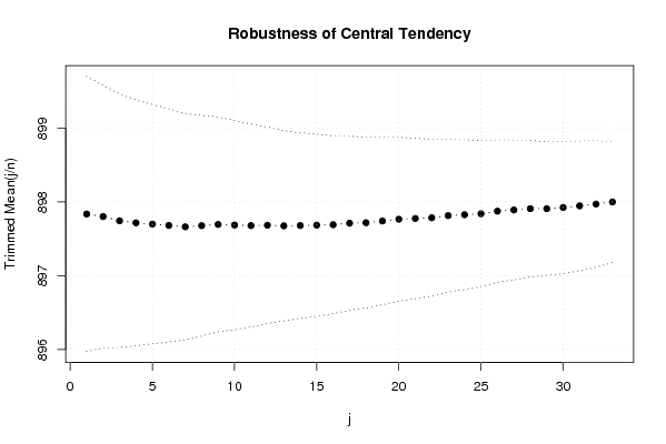
bitmap(file='test2.png')
lb <- tri[,1] - 2*tri[,2]
ub <- tri[,1] + 2*tri[,2]
if ((ylimmin == '') | (ylimmax == '')) plot(tri[,1],type='b',main='Robustness of Central Tendency', xlab='j', pch=19, ylab='Trimmed Mean(j/n)', ylim=c(min(lb),max(ub))) else plot(tri[,1],type='l',main='Robustness of Central Tendency', xlab='j', pch=19, ylab='Trimmed Mean(j/n)', ylim=c(ylimmin,ylimmax))
lines(ub,lty=3)
lines(lb,lty=3)
grid()
dev.off()
a<-table.start()
a<-table.row.start(a)
a<-table.element(a,'Central Tendency - Ungrouped Data',4,TRUE)
a<-table.row.end(a)
a<-table.row.start(a)
a<-table.element(a,'Measure',header=TRUE)
a<-table.element(a,'Value',header=TRUE)
a<-table.element(a,'S.E.',header=TRUE)
a<-table.element(a,'Value/S.E.',header=TRUE)
a<-table.row.end(a)
a<-table.row.start(a)
a<-table.element(a,hyperlink('arithmetic_mean.htm', 'Arithmetic Mean', 'click to view the definition of the Arithmetic Mean'),header=TRUE)
a<-table.element(a,arm)
a<-table.element(a,hyperlink('arithmetic_mean_standard_error.htm', armse, 'click to view the definition of the Standard Error of the Arithmetic Mean'))
a<-table.element(a,armose)
a<-table.row.end(a)
a<-table.row.start(a)
a<-table.element(a,hyperlink('geometric_mean.htm', 'Geometric Mean', 'click to view the definition of the Geometric Mean'),header=TRUE)
a<-table.element(a,geo)
a<-table.element(a,'')
a<-table.row.end(a)
a<-table.row.start(a)
a<-table.element(a,hyperlink('harmonic_mean.htm', 'Harmonic Mean', 'click to view the definition of the Harmonic Mean'),header=TRUE)
a<-table.element(a,har)
a<-table.element(a,'')
a<-table.row.end(a)
a<-table.row.start(a)
a<-table.element(a,hyperlink('quadratic_mean.htm', 'Quadratic Mean', 'click to view the definition of the Quadratic Mean'),header=TRUE)
a<-table.element(a,qua)
a<-table.element(a,'')
a<-table.row.end(a)
for (j in 1:length(win[,1])) {
a<-table.row.start(a)
mylabel <- paste('Winsorized Mean (',j)
mylabel <- paste(mylabel,'/')
mylabel <- paste(mylabel,length(win[,1]))
mylabel <- paste(mylabel,')')
a<-table.element(a,hyperlink('winsorized_mean.htm', mylabel, 'click to view the definition of the Winsorized Mean'),header=TRUE)
a<-table.element(a,win[j,1])
a<-table.element(a,win[j,2])
a<-table.element(a,win[j,1]/win[j,2])
a<-table.row.end(a)
}
for (j in 1:length(tri[,1])) {
a<-table.row.start(a)
mylabel <- paste('Trimmed Mean (',j)
mylabel <- paste(mylabel,'/')
mylabel <- paste(mylabel,length(tri[,1]))
mylabel <- paste(mylabel,')')
a<-table.element(a,hyperlink('arithmetic_mean.htm', mylabel, 'click to view the definition of the Trimmed Mean'),header=TRUE)
a<-table.element(a,tri[j,1])
a<-table.element(a,tri[j,2])
a<-table.element(a,tri[j,1]/tri[j,2])
a<-table.row.end(a)
}
a<-table.row.start(a)
a<-table.element(a,hyperlink('median_1.htm', 'Median', 'click to view the definition of the Median'),header=TRUE)
a<-table.element(a,median(x))
a<-table.element(a,'')
a<-table.row.end(a)
a<-table.row.start(a)
a<-table.element(a,hyperlink('midrange.htm', 'Midrange', 'click to view the definition of the Midrange'),header=TRUE)
a<-table.element(a,midr)
a<-table.element(a,'')
a<-table.row.end(a)
a<-table.row.start(a)
mymid <- hyperlink('midmean.htm', 'Midmean', 'click to view the definition of the Midmean')
mylabel <- paste(mymid,hyperlink('method_1.htm','Weighted Average at Xnp',''),sep=' - ')
a<-table.element(a,mylabel,header=TRUE)
a<-table.element(a,midm[1])
a<-table.element(a,'')
a<-table.row.end(a)
a<-table.row.start(a)
mymid <- hyperlink('midmean.htm', 'Midmean', 'click to view the definition of the Midmean')
mylabel <- paste(mymid,hyperlink('method_2.htm','Weighted Average at X(n+1)p',''),sep=' - ')
a<-table.element(a,mylabel,header=TRUE)
a<-table.element(a,midm[2])
a<-table.element(a,'')
a<-table.row.end(a)
a<-table.row.start(a)
mymid <- hyperlink('midmean.htm', 'Midmean', 'click to view the definition of the Midmean')
mylabel <- paste(mymid,hyperlink('method_3.htm','Empirical Distribution Function',''),sep=' - ')
a<-table.element(a,mylabel,header=TRUE)
a<-table.element(a,midm[3])
a<-table.element(a,'')
a<-table.row.end(a)
a<-table.row.start(a)
mymid <- hyperlink('midmean.htm', 'Midmean', 'click to view the definition of the Midmean')
mylabel <- paste(mymid,hyperlink('method_4.htm','Empirical Distribution Function - Averaging',''),sep=' - ')
a<-table.element(a,mylabel,header=TRUE)
a<-table.element(a,midm[4])
a<-table.element(a,'')
a<-table.row.end(a)
a<-table.row.start(a)
mymid <- hyperlink('midmean.htm', 'Midmean', 'click to view the definition of the Midmean')
mylabel <- paste(mymid,hyperlink('method_5.htm','Empirical Distribution Function - Interpolation',''),sep=' - ')
a<-table.element(a,mylabel,header=TRUE)
a<-table.element(a,midm[5])
a<-table.element(a,'')
a<-table.row.end(a)
a<-table.row.start(a)
mymid <- hyperlink('midmean.htm', 'Midmean', 'click to view the definition of the Midmean')
mylabel <- paste(mymid,hyperlink('method_6.htm','Closest Observation',''),sep=' - ')
a<-table.element(a,mylabel,header=TRUE)
a<-table.element(a,midm[6])
a<-table.element(a,'')
a<-table.row.end(a)
a<-table.row.start(a)
mymid <- hyperlink('midmean.htm', 'Midmean', 'click to view the definition of the Midmean')
mylabel <- paste(mymid,hyperlink('method_7.htm','True Basic - Statistics Graphics Toolkit',''),sep=' - ')
a<-table.element(a,mylabel,header=TRUE)
a<-table.element(a,midm[7])
a<-table.element(a,'')
a<-table.row.end(a)
a<-table.row.start(a)
mymid <- hyperlink('midmean.htm', 'Midmean', 'click to view the definition of the Midmean')
mylabel <- paste(mymid,hyperlink('method_8.htm','MS Excel (old versions)',''),sep=' - ')
a<-table.element(a,mylabel,header=TRUE)
a<-table.element(a,midm[8])
a<-table.element(a,'')
a<-table.row.end(a)
a<-table.row.start(a)
a<-table.element(a,'Number of observations',header=TRUE)
a<-table.element(a,length(x))
a<-table.element(a,'')
a<-table.row.end(a)
a<-table.end(a)
table.save(a,file='mytable.tab')
a<-table.start()
a<-table.row.start(a)
a<-table.element(a,'Variability - Ungrouped Data',2,TRUE)
a<-table.row.end(a)
for (i in 1:num) {
a<-table.row.start(a)
if (res[i,1] != '') {
a<-table.element(a,hyperlink(res[i,2],res[i,1],''),header=TRUE)
} else {
a<-table.element(a,res[i,2],header=TRUE)
}
a<-table.element(a,res[i,3])
a<-table.row.end(a)
}
a<-table.end(a)
table.save(a,file='mytable1.tab')
lx <- length(x)
qval <- array(NA,dim=c(99,8))
mystep <- 25
mystart <- 25
if (lx>10){
mystep=10
mystart=10
}
if (lx>20){
mystep=5
mystart=5
}
if (lx>50){
mystep=2
mystart=2
}
if (lx>=100){
mystep=1
mystart=1
}
for (perc in seq(mystart,99,mystep)) {
qval[perc,1] <- q1(x,lx,perc/100,i,f)
qval[perc,2] <- q2(x,lx,perc/100,i,f)
qval[perc,3] <- q3(x,lx,perc/100,i,f)
qval[perc,4] <- q4(x,lx,perc/100,i,f)
qval[perc,5] <- q5(x,lx,perc/100,i,f)
qval[perc,6] <- q6(x,lx,perc/100,i,f)
qval[perc,7] <- q7(x,lx,perc/100,i,f)
qval[perc,8] <- q8(x,lx,perc/100,i,f)
}
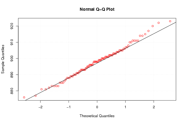
bitmap(file='test3.png')
myqqnorm <- qqnorm(x,col=2)
qqline(x)
grid()
dev.off()
a<-table.start()
a<-table.row.start(a)
a<-table.element(a,'Percentiles - Ungrouped Data',9,TRUE)
a<-table.row.end(a)
a<-table.row.start(a)
a<-table.element(a,'p',1,TRUE)
a<-table.element(a,hyperlink('method_1.htm', 'Weighted Average at Xnp',''),1,TRUE)
a<-table.element(a,hyperlink('method_2.htm','Weighted Average at X(n+1)p',''),1,TRUE)
a<-table.element(a,hyperlink('method_3.htm','Empirical Distribution Function',''),1,TRUE)
a<-table.element(a,hyperlink('method_4.htm','Empirical Distribution Function - Averaging',''),1,TRUE)
a<-table.element(a,hyperlink('method_5.htm','Empirical Distribution Function - Interpolation',''),1,TRUE)
a<-table.element(a,hyperlink('method_6.htm','Closest Observation',''),1,TRUE)
a<-table.element(a,hyperlink('method_7.htm','True Basic - Statistics Graphics Toolkit',''),1,TRUE)
a<-table.element(a,hyperlink('method_8.htm','MS Excel (old versions)',''),1,TRUE)
a<-table.row.end(a)
for (perc in seq(mystart,99,mystep)) {
a<-table.row.start(a)
a<-table.element(a,round(perc/100,2),1,TRUE)
for (j in 1:8) {
a<-table.element(a,round(qval[perc,j],6))
}
a<-table.row.end(a)
}
a<-table.end(a)
table.save(a,file='mytable2.tab')
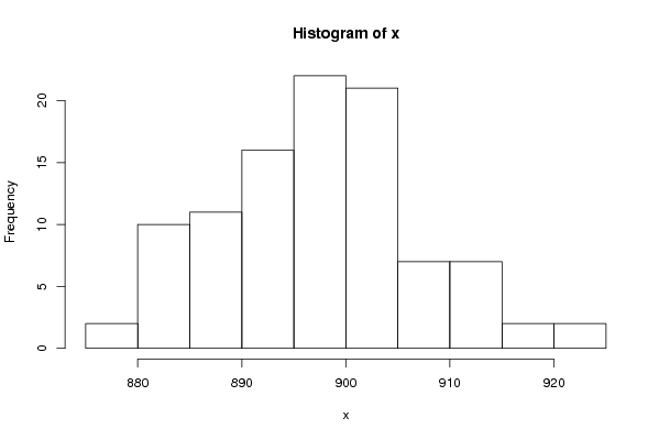
bitmap(file='histogram1.png')
myhist<-hist(x)
dev.off()
myhist
n <- length(x)
a<-table.start()
a<-table.row.start(a)
a<-table.element(a,hyperlink('histogram.htm','Frequency Table (Histogram)',''),6,TRUE)
a<-table.row.end(a)
a<-table.row.start(a)
a<-table.element(a,'Bins',header=TRUE)
a<-table.element(a,'Midpoint',header=TRUE)
a<-table.element(a,'Abs. Frequency',header=TRUE)
a<-table.element(a,'Rel. Frequency',header=TRUE)
a<-table.element(a,'Cumul. Rel. Freq.',header=TRUE)
a<-table.element(a,'Density',header=TRUE)
a<-table.row.end(a)
crf <- 0
mybracket <- '['
mynumrows <- (length(myhist$breaks)-1)
for (i in 1:mynumrows) {
a<-table.row.start(a)
if (i == 1)
dum <- paste('[',myhist$breaks[i],sep='')
else
dum <- paste(mybracket,myhist$breaks[i],sep='')
dum <- paste(dum,myhist$breaks[i+1],sep=',')
if (i==mynumrows)
dum <- paste(dum,']',sep='')
else
dum <- paste(dum,mybracket,sep='')
a<-table.element(a,dum,header=TRUE)
a<-table.element(a,myhist$mids[i])
a<-table.element(a,myhist$counts[i])
rf <- myhist$counts[i]/n
crf <- crf + rf
a<-table.element(a,round(rf,6))
a<-table.element(a,round(crf,6))
a<-table.element(a,round(myhist$density[i],6))
a<-table.row.end(a)
}
a<-table.end(a)
table.save(a,file='mytable5.tab')
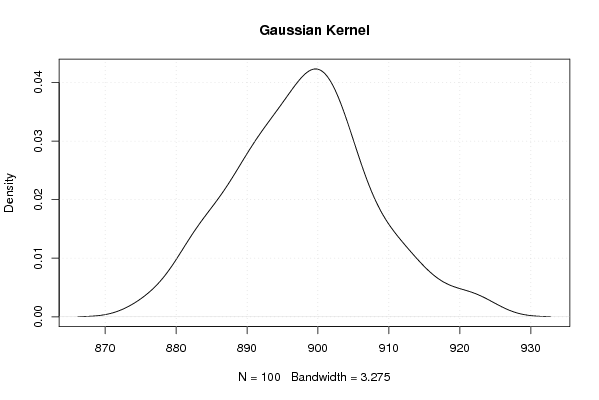
bitmap(file='density1.png')
mydensity1<-density(x,kernel='gaussian',na.rm=TRUE)
plot(mydensity1,main='Gaussian Kernel')
grid()
dev.off()
mydensity1
a<-table.start()
a<-table.row.start(a)
a<-table.element(a,'Properties of Density Trace',2,TRUE)
a<-table.row.end(a)
a<-table.row.start(a)
a<-table.element(a,'Bandwidth',header=TRUE)
a<-table.element(a,mydensity1$bw)
a<-table.row.end(a)
a<-table.row.start(a)
a<-table.element(a,'#Observations',header=TRUE)
a<-table.element(a,mydensity1$n)
a<-table.row.end(a)
a<-table.end(a)
table.save(a,file='mytable4.tab')